Ex_014 Analytical Permeability Models

Contents
In the current tutorial example we present the data input required to use the analytical porosity-permeability models in ParaGeo. In addition we provide an excel spreadsheet in which:
1.The user may visualise the expected porosity vs. permeability curve for all the implemented models and any input values.
2.We validate the results obtained from the simulation examples provided here against the analytical permeability calculated for each porosity value output in the history point.
The data and results are provided in ParaGeo_Examples/Ex_014.
The data files provided consider vertical compressional displacement of 0.7 m magnitude applied on a 1 x 1 x 1 m cube of sediment. Because the initial porosity is defined as 0.7, the results will cover the whole porosity range for the defined material. The results will be output at a history point located at the centre of the cube. The file is set up as a coupled simulation (required to output the permeability) but with pore pressure fully prescribed (with zero value).
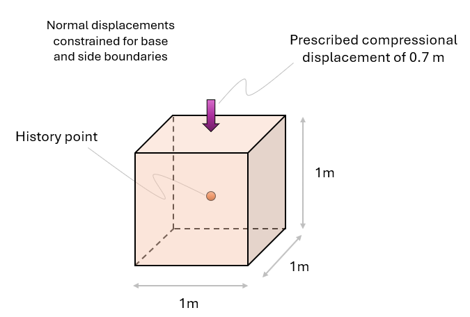
Schematic of model geometry
Five cases are considered:
•Case01a: Power Law
•Case01b: Power Law (with anisotropy and perm cutoffs)
•Case02: Kozeny-Carman (with anisotropy)
•Case03: Exponential model (with anisotropy)
•Case04: Yang and Aplin model (with anisotropy)
Note that in Cases 02, 03 and 04 the data include the keywords defining minimum and maximum permeability cutoffs but are set with values such that they do not have any effect on the predicted permeability.
The data input for each case is demonstrated in the following sections. Note that only the data defining the permeability models will be shown and discussed.
In the plots shown below, extra porosity-permeability curves are displayed for reference; i.e:
1.Typical Sandstone, Siltstone and Shale Kozeny-Carman curves according to Hantschel and Kauerauf (2009). Note that those curves use a revised form of Kozeny-Carman proposed by Ungerer et al. (1990) whereas the model available in ParaGeo is the original Kozeny-Carman model.
2.Yang and Aplin curves for clay fractions of 0.0, 0.2, 0.4, 0.6, 0.8 and 1.0 are shown in discontinuous grey lines.
Case01a Power Law (isotropic)
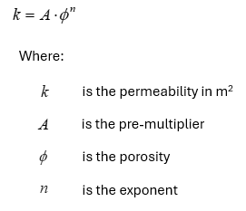
In Case01a a Power Law function as shown below is used:
Data file |
|
* Material_data ! --------------------------------- Name "Shale" ! --------------------------------- Permeability_type 5 Permeability_properties IDM=2 /"A"/ 1E-12 /"n"/ 8 |
1.Permeability_type set to 5 uses the Power Law function.
2.Two input properties are required: a.Pre-multiplier (A) b.Exponent (n)
|
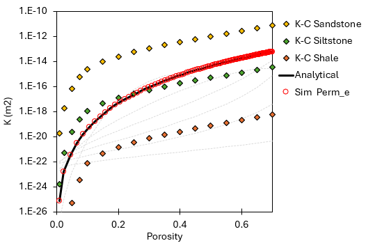
Case01a: Comparison of simulated vs analytical permeability as a function of porosity.
Case01b Power Law (with anisotropy and perm cutoffs)
In Case01b the same Power Law function as in Case01a is used, but adding extra keywords to consider minimum and maximum permeability cutoff values and permeability anisotropy (where horizontal permeabilities are a factor of the vertical permeability).
Data file |
|
* Material_data ! --------------------------------- Name "Shale" ! --------------------------------- Permeability_type 5 Permeability_properties IDM=2 /"A"/ 1E-12 /"n"/ 8 Max_permeability_cutoff 1E-14 Min_permeability_cutoff 1E-21 Perm_anisotropy_factor 2.0 ! ---------------------------------
|
1.The same power law function as in Case01a is used.
2.Max_permeability_cutoff and Min_permeability_cutoff keywords are used to constrain the allowable range of permeabilities. This might be useful in some circumstances to ensure numerical stability by avoiding extreme values which may not have a meaningful impact on the solution.
3.Perm_anisotropy_factor is set as 2.0. This will consider transverse isotropic permeability in which horizontal permeabilities will be 2 times the vertical permeability.
4.Note that isotropic and anisotropic permeabilities use different state variables so that the output variables are defined accordingly for the history point:
▪Perm_e : Isotropic permeability ▪Perm_x, Perm_y and Perm_z : Permeability in the X, Y and Z directions respectively (for anisotropic perm) |
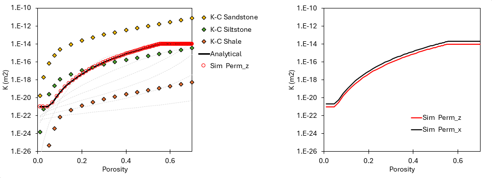
Case01b: Comparison of simulated vs analytical permeability as a function of porosity (left). Simulated vertical and horizontal permeabilities (right).
Case02 Kozeny-Carman model
In Case02 the classical Kozeny-Carman model is used. This is described by the function:
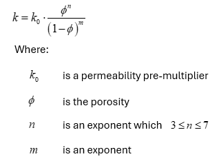
In the bibliography the pre-multiplier (k0) may be defined according to pore-geometry considerations:
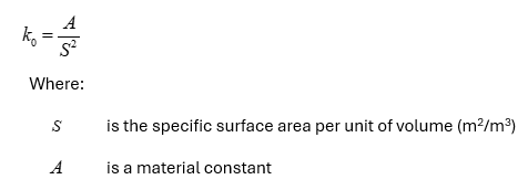
However in ParaGeo the pre-multiplier is directly input for the sake of simplicity.
Data file |
|
* Material_data ! --------------------------------- Name "Shale" ! --------------------------------- Permeability_type 6 Permeability_properties IDM=3 /"Pre-multiplier"/ 1E-15 /"Exponent n"/ 3 /"Exponent m"/ 2 Max_permeability_cutoff 1E-12 Min_permeability_cutoff 1E-24 Perm_anisotropy_factor 2.0 ! ---------------------------------
|
1.Permeability_type set to 6 uses the Kozeny-Carman model.
2.Three input properties are required: a.Pre-multiplier (k0) b.Exponent (n) c.Exponent (m)
3.Max_permeability_cutoff and Min_permeability_cutoff keywords are defined with values such that they do not constrain the range of permeabilities for the chosen input values.
4.Perm_anisotropy_factor is set as 2.0. This will consider transverse isotropic permeability in which horizontal permeabilities will be 2 times the vertical permeability. |
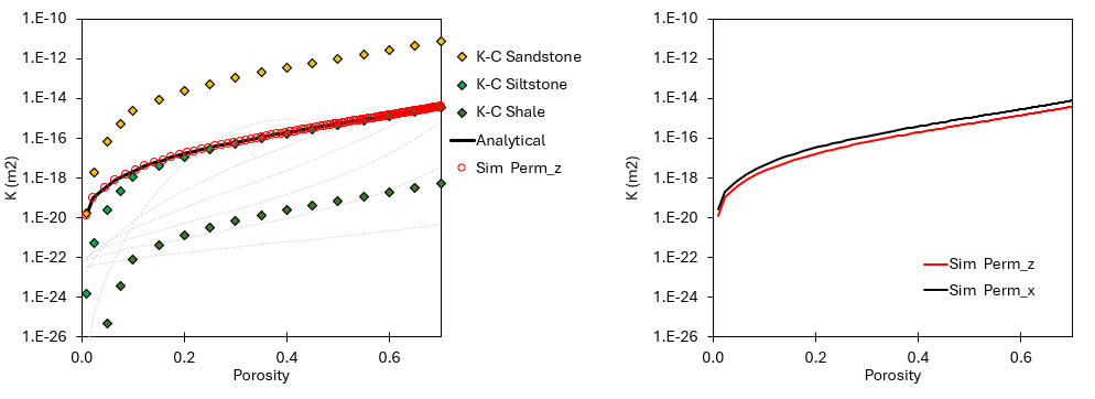
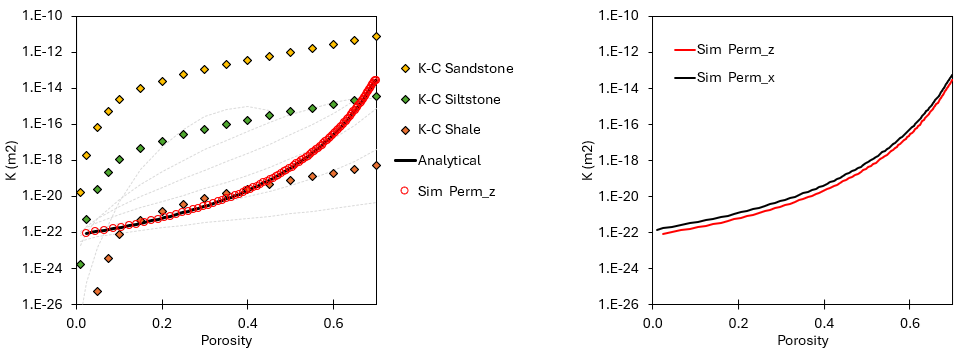
Case02: Comparison of simulated vs analytical permeability as a function of porosity (left). Simulated vertical and horizontal permeabilities (right).
Case03 Exponential Law
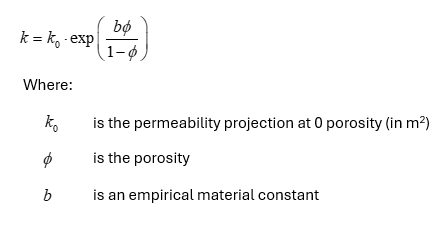
In Case03 the Exponential law is used (e.g. Nygård et al (2004)) . This is described by the function:
Data file |
|
* Material_data ! --------------------------------- Name "Shale" ! --------------------------------- Permeability_type 7 Permeability_properties IDM=2 /"k0"/ 5.72E-23 /"b"/ 8.57 Max_permeability_cutoff 1E-12 Min_permeability_cutoff 1E-24 Perm_anisotropy_factor 2.0 ! ---------------------------------
|
1.Permeability_type set to 7 uses the Exponential law.
2.Two input properties are required: a.Pre-multiplier (k0) b.Material constant (b)
3.Max_permeability_cutoff and Min_permeability_cutoff keywords are defined with values such that they do not constrain the range of permeabilities for the chosen input values.
4.Perm_anisotropy_factor is set as 2.0. This will consider transverse isotropic permeability in which horizontal permeabilities will be 2 times the vertical permeability. |
Case03: Comparison of simulated vs analytical permeability as a function of porosity (left). Simulated vertical and horizontal permeabilities (right).
Case04 Yang and Aplin model
In Case04 the Yang and Aplin model is used. This model is derived from experimental results to predict the permeability in shales based on the clay fraction (C.F.) content:
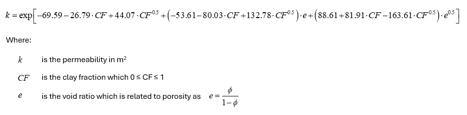
Data file |
|
* Material_data ! --------------------------------- Name "Shale" ! --------------------------------- Permeability_type 8 Permeability_properties IDM=1 /"C.F."/ 0.7 Max_permeability_cutoff 1E-12 Min_permeability_cutoff 1E-24 Perm_anisotropy_factor 2.0 ! --------------------------------- |
1.Permeability_type set to 8 uses the Yang and Aplin model.
2.A single input property is required: a.Clay Fraction (C.F.)
3.Max_permeability_cutoff and Min_permeability_cutoff keywords are defined with values such that they do not constrain the range of permeabilities for the chosen input values.
4.Perm_anisotropy_factor is set as 2.0. This will consider transverse isotropic permeability in which horizontal permeabilities will be 2 times the vertical permeability. |
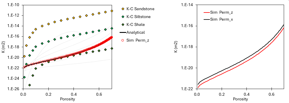
Case04: Comparison of simulated vs analytical permeability as a function of porosity (left). Simulated vertical and horizontal permeabilities (right).