Overview

The objective is to re-perform the simulation using the permeability (k) = 1.0E-19m2.  This is achieved by defining a new material in the hm_002_elastic.mat file called hm_002_elastic_1E19 and then changing the data file to read this data.  The example data is provided in HM_003\Exercises\Case 2\Data. The case with the linear sedimentation time curve is hm_003_Case2.dat and hm_003_Case2a.dat is the S-Curve sedimentation time curve case.

 

Results

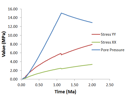
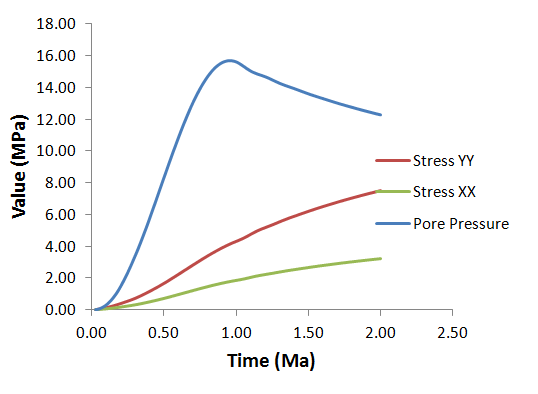
The result files for the project are in directory: HM_002\Exercises\Case 2\results and the high definition history files can be displayed in excel file hm_003_Case3.xlsx.   The evolution of pore pressure and effective stress are shown below.   The predicted maximum overpressure at the base of the column is ca. 5.3 MPa for hm_003_Case3 and ca. 5,4 Ma for hm_003_Case3.  These values are very close to the analytical solution.

Effective Vertical/Horizontal Stress and Pore Pressure as a Function of Time

Comparison of the pore pressure vs. time curves for the two cases show that they are almost identical in the post-sedimentation phase between t = 1.1 and t = 2.0s.

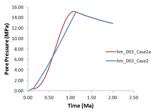
Comparison of the Predicted Pore Pressure Evolution for Case 2 and Case 2A

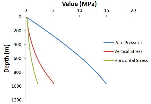
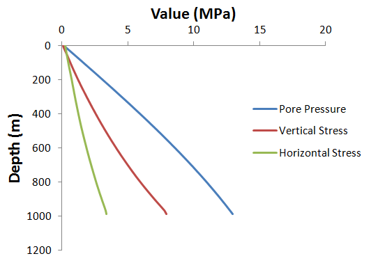
The graphs of pore pressure, vertical effective stress and horizontal effective stress as a function of depth are created by exporting data for "graph on a line" from ParaView at time t = 1.0 Ma and t = 2.0 Ma.   Due to the large overpressure the effective stresses at time t=1,0 Ma are very low but increase significantly by time t = 2.0 Ma.

Effective Vertical/Horizontal Stress and Pore Pressure as a Function of Depth

 

The predicted overpressure profile as a function of depth at t = 1.0Ma is very close to the analytical solution.  An exact match is not expected due to the slightly different loading regimes in the analytical model and the simulation.

 

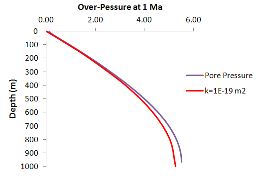
Comparison of the Predicted Pore Pressure and the Analytical Solution at time t = 1.0 Ma