Introduction to the intersect Model
Introduction to the intersect Model
Intersect (IX) is Chevron’s next generation reservoir simulator. Intersect is an adaptive-implicit black oil, compositional, and thermal simulator based on next-generation architecture. It is being developed under a multi-year collaborative project involving Chevron, Schlumberger, and Total. It offers improved performance and scalability that makes it ideal for large and highly heterogeneous simulation models with complex grid geometries. Another benefit is the flexible field management system.
This section describes the various reservoir simulation components in Intersect and the set-up of the training models.

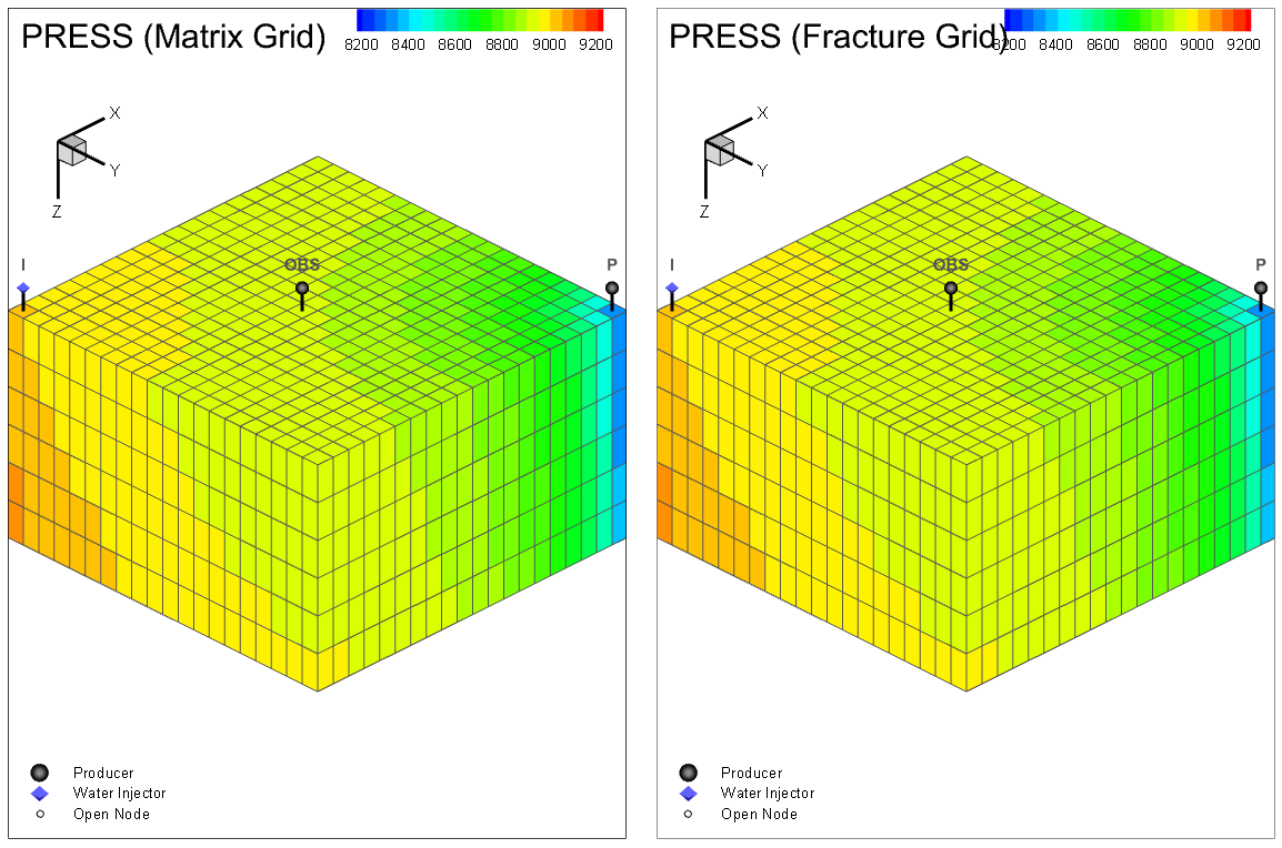
3D model view of IX dual porosity dual permeability model
INTERSECT™ is a trademark of Schlumberger Technology Corporation. INTERSECT software is a joint product collaboration of Chevron U.S.A. Inc., TOTAL E&P Services, and Schlumberger Technology Corporation.
Reservoir Simulation
Overarching model
The primary INTERSECT input file is an AFI file. This top level file has a text format and contains a list of the associated input files or directories to include for each simulation. The structure of the file in this example is as follows:
Within the *.afi file, the *.ixf files are the include files containing input data for the reservoir simulator and for Field Management. The ixf format is a text-based input file format that can also be read, understood and manually edited.
In this example, we have also requested that IX report an extended GRID file that can then be imported in Petrel or TecPlot for visualization. There is a further command required in the reservoir section.
There are two main sections in an INTERSECT model:
1.The reservoir section:
a. The fluid PVT define the properties of the hydrocarbon phase and water in the reservoir. b.The rock properties define the relative permeability tables used for multiphase flow calculations as well as rock compressibility table. c.The initialization data include the fluid contacts, initial pressure and temperature conditions while the region data allocates fluid/rock/initialisation data to specific ranges of grid blocks. d.The wells contain the information on well path and completion types
2.The field management section:
a.The well control parameters define the well constrains (e.g. flow rates, minimum or maximum pressure) and well types. b.The production strategy specifies the sequence of actions for wells coming online, for guide rate balancing or reservoir pressure targets. c.The recurrent reporting fields specifies the entities and quantities reported at regular intervals for either wells or 3D cells. d.The coupling include IXF file is highlighted in yellow and is described in IX Coupling Files page.
|
Static Geologic Model
Users can define grid geometry directly in ASCII text in IXF, using the node StraightPillarGrid, instead of using a GSG grid file. This enables engineers to quickly define a simple grid for a simple model, for example, one dimensional cores, slim tubes, etc.
In this tutorial we use three different models:
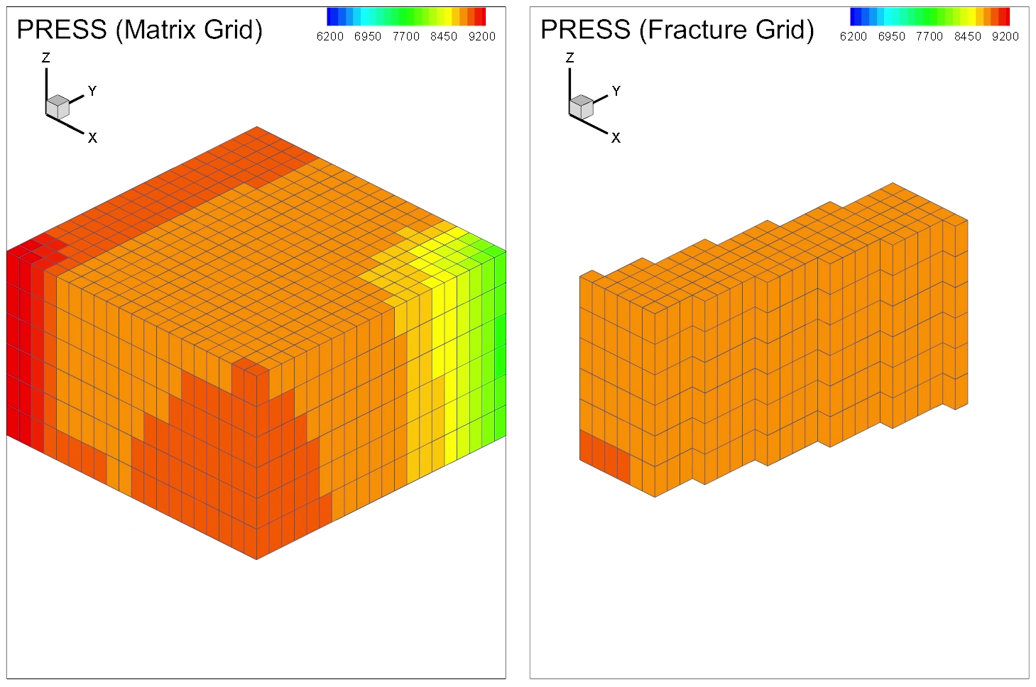
1.Single Porosity 2.Dual Porosity 3.Dual Porosity Corridor
All models use the same geometry to allow for better comparison between the various geological realisations. The basic set-up uses a simple box model with dimensions 20, 20 and 6 in the X, Y and Z directions. The dimensions of each gridblock are 125 ft, 125 ft and 25 ft in the the X-, Y- and Z- direction respectively. The top of the reservoir is located 14,765 ft deep.
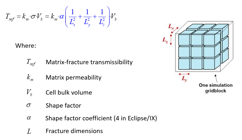
The original model was 5 times finer in all directions resulting an overall model size of 300,000 cells in the matrix system. For the purpose of running the model as part of a training exercise, it was decided to use a coarser version of this model that would run faster. The current coarse model has 2400 cells in the matrix. The resulting run time is in the order of minutes instead of hours. An important consideration when upscaling the model was to retain the dynamic behaviour of the coarse model is consistent with the finer scale model. In this configuration, the grid is left handed.
|
Rock Properties
The relative permeability and capillary pressure description consists of both drainage and imbibition curves. INTERSECT is using a three-phase description with oil, gas and water phases being present. The relative permeability and capillary pressure data are input as tables.
An important comment to make here is the need for consistency between the matrix pore volume compressibility defined in INTERSECT and the mechanical rock properties defined in ParaGeo.
A simple relationship that can be used that relates rock compressibility (
Or inversely:
|
Fluid Properties
The fluid description is compositional. The model uses a Peng-Robinson type cubic equation of state. The inputs required include individual component properties, binary interaction coefficients, volume shift and omega values used in the definition of the attractive and covolume parameters.
|
Initialisation and Region Mapping
The datum depth in this example is set as the top of the reservoir (14765ft TVDss). The reservoir is 150 ft thick and positioned within the oil leg. The Oil-Water contact is much deeper with no transition zone effects expected in the model. The initial reservoir pressure is 11950 psi at datum depth. The composition of the fluid is specified under the Equilibrium node and has no compositional gradient with depth. There is however a temperature vs depth table defined to capture the geothermal gradient in the reservoir.
|
Well Model and Completions
The final component of the reservoir section is the definition of the wells. The model is a simple quarter symmetry box model with three (3) wells. The injector [“I”] and producer [“PROD”] wells are defined in opposite corners of the model ( [1 1] vs [20 20]). In addition, an observation [“OBS”] well has been added to monitor the pressure half-way between the wells. All wells are vertical and completed along the K axis. The wellbore radius is 0.25ft. The productivity index (PI) of the well is kept at its calculated value with a multiplier of 1.0.
Depending on the geological realization, the wells are completed either in the matrix or in both the matrix and fracture cells.
|
Field Management
Well Control
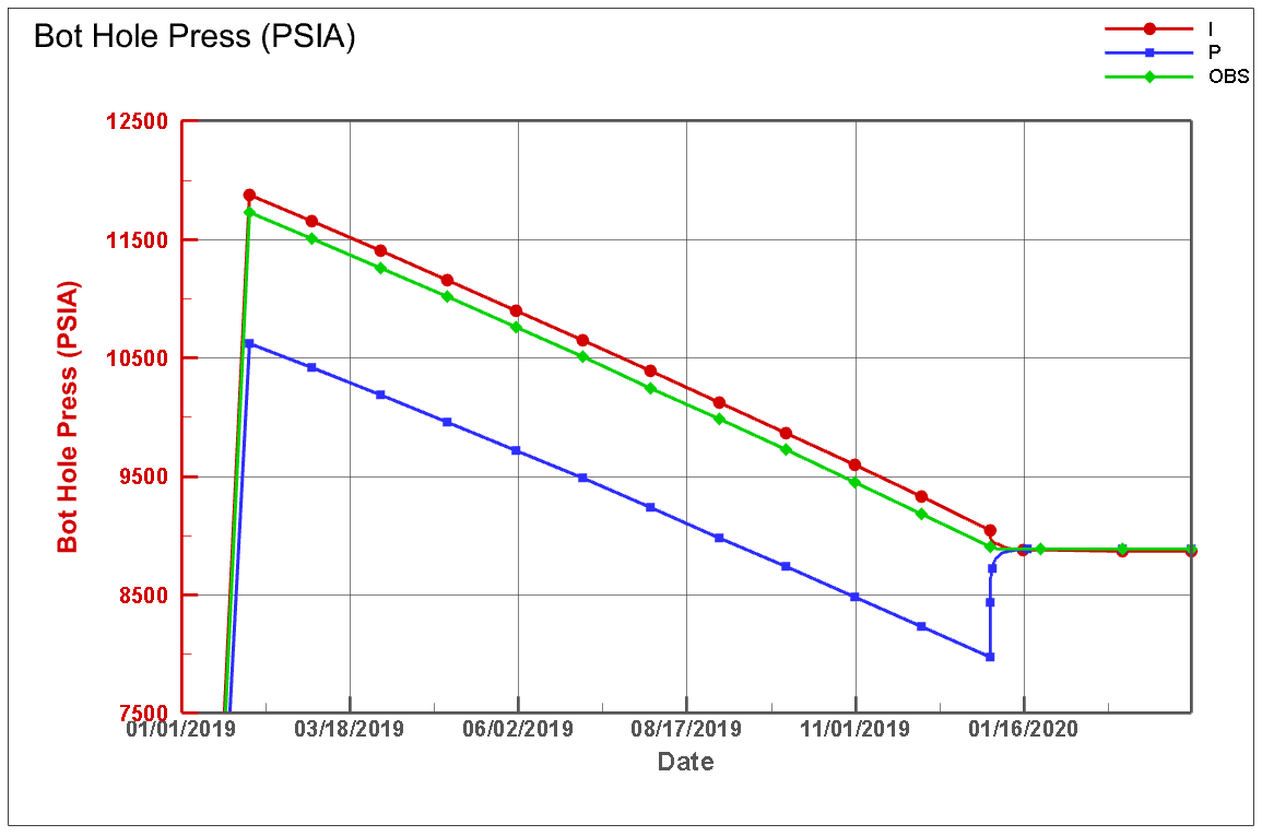
In this exercise, the reservoir is being produced with a voidage replacement ratio lower than 1. The voidage replacement ratio is defined as the volume of injected fluid to the volume of the produced fluid. The production rate has been set at 15000 rb/d and the water injection at a limited 1000 rb/d. The rationale for such an imbalance in the production system is to create a significant amount of depletion in the model over a short period of time. The observation well has also been assigned a production rate to allow for the well pressure to be resolved. The rate is insignificant so that it does not interfere with the fluid flow.
|
Schedule and Production Strategy
The production system is operated under mainly depletion with a little injection. This is carried out for a period of 12 months. For the next 3 months, the wells are shut-in with very fine timesteps as if to model a DST response of a build-up test. There is no complex production strategy defined in this model. The wells are simply controlled on reservoir volume rate. It is however possible to assign specific voidage replacement constraints (e.g. GuideRateBalanceAction) or pressure targets (e.g. PIDControl) to the model as and if required by the study objectives.
|
Initial and Recurrent Data
The field management section in IX includes specific reports for the initial static properties and for the time dependent dynamic entities within the 3D grid. The values are stored for each individual gridblock in the *.INIT and *.UNRST files. The frequency and period (i.e. every n-th report) can be specified.
Non-standard keywords have been added specifically for the purpose of linking reservoir simulation models (INTERSECT) to mechanical Earth models (ParaGeo).
•New objects containing a pointer to the X-, Y-, and Z-direction displacement arrays on IX cell centers have been created. These arrays are only used for output of displacements on reservoir grid in IX recurrent 3D report (corresponding IX property names are DISPX, DISPY, DISPZ).
•New objects containing a pointer to the XX-, YY-, ZZ-, XY-, XZ-, and YZ- component stress arrays on IX cell centers have been added. These arrays are only used for output of stresses on reservoir grid in IX recurrent 3D report (corresponding IX property names are STRESSXX, STRESSYY, STRESSZZ, STRESSXY, STRESSXZ, STRESSYZ).
•New strain objects containing a pointer to the XX-, YY-, ZZ-, XY-, XZ-, YZ- component and vertical strain arrays on IX cell centers are also available . These arrays are only used for output of strains on reservoir grid in IX recurrent 3D report (corresponding IX property names are STRNXX, STRNYY, STRNZZ, STRNXY, STRNXZ, STRNYZ, VSTRAIN).
The performance of individual wells, groups of wells or the field as a whole can be reported using “XYPlotSummaryReport” functionality. This is very useful for plotting entities as a function of time, e.g. flow rates of well pressure.
The same functionality can be used to report specific cell properties as a function of time. The following commands are used to extract the cell property at the well locations ([1 1], [20 20] and [10 10]). The cells are located in layer 3, i.e. 3 and 9 in the matrix and the fracture systems respectively. As for the grid report, the SelectedProperties correspond to the IX internal entities, while the ReportLabels are the names found in the output files.
Example of pressure response for the CellProperties report
|
Time Controls
The start date of the simulation is specified in the Field Management section using the FieldManagement { } keyword. The target times for reporting or changing well constraints are then added after the START command with the DATE keyword. In this example, the format is “dd-mmm-yyyy hh:mm:ss”.
|
Two-Way Coupling Controls
The last IXF file in this model is the user extension file used as part of the two-way coupling workflow. The file provides the control parameters for the API linking INTERSECT to ParaGeo. The various commands are discussed in IX Coupling Files page.
|


