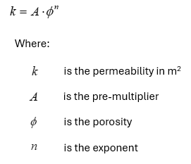
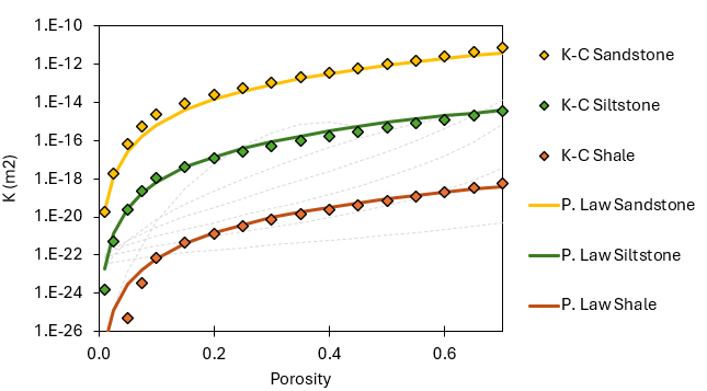
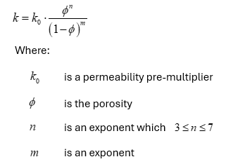
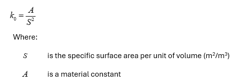
Material_data
Data Structure: Material_data |
|
Description |
Material data structure |
Usage |
Material_data NUM=ival where ival is the data structure number |
Description |
||||||||||||||||||||||||||||||||||||||||||||||||||||
Overview The Material_data structure defines all material properties directly related to the solid or porous medium for all fields. The data required is dependent on the active fields and on the particular analysis options and material models selected for those fields. Typical usage includes:
All Fields
Geomechanical Field
Porous Field
Thermal Field
Notes •Several Material_data structure may be defined.
Examples All examples require specification of the Material_data structure with the exception of mesh generation examples where no analysis is performed.
|
| Name (or Material_name) Material name |
Usage |
||||
|
||||
Description |
||||
Material name (maximum 128 characters)
|
| Mdb_class Material class name (Optional, Compulsory if material data is to be imported from a database) |
Usage |
||||
|
||||
Description |
||||
The name of the material database class; i.e. the directory name in the PARAGEOHOME/MDB directory (maximum 128 characters).
Notes •If material data is to be imported from a database the Mdb_class and Mdb_name must be specified either in the Mdb_control_data or Material_data structures.
|
| Mdb_name Material database name (Optional, Compulsory if material data is to be imported from a database) |
Usage |
||||
|
||||
Description |
||||
The name of the material database; i.e. the file name in the PARAGEOHOME/MDB/Mdb_class directory (maximum 128 characters).
Notes •The material database must have extension .mdb but may be defined in the data file with or without the extension •If material data is to be imported from a database the Mdb_class and Mdb_name must be specified either in the Mdb_control_data or Material_data structures.
|
| Mdb_material_name Material nae in database (Optional) |
Usage |
||||
|
||||
Description |
||||
The name of the material in the database Mdb_name (maximum 128 characters). By default the material name is assumed to be the same as the material name specified by the Name keyword.
Notes •If material data is to be imported from a database the Mdb_class and Mdb_name must be specified either in the Mdb_control_data or Material_data structures.
|
| Material_file Local .mat file name for import (Optional) |
Usage |
||||
|
||||
Description |
||||
Mat_file_name allows the import of material data from a local .mat file. If the .mat file contains more than one material then the Name (if specified) or Mdb_material_name will be used to extract the data. The material name will be the name specified by Name keyword in the data file (if specified). If the Material_name keyword is not specified in the data file the Name defined in the .mat file will be used.
Notes •The material file name must have extension .mat but may be defined in the data file with or without the extension
|
| Description Material description (Optional) |
Usage |
||||
|
||||
Description |
||||
Description of material (maximum of 1028 characters)
|
| Reference_temperature Reference temperature for material properties |
Usage |
||||
|
||||
Description |
||||
Reference temperature for material properties
|
| Gas_constant Universal gas constant |
Usage |
||||
|
||||
Description |
||||
Universal gas constant. If the gas constant is not specified it will be automatically evaluated dependent on the standard units defined by Units.
|
| Units Units used to define the material properties (Optional) |
Usage |
|||||||||||||||
|
|||||||||||||||
Description |
|||||||||||||||
Units used to define the material properties. Vector dimensioned 4 where: •Location 1 - units for stress e.g. ("MPa", "KPa", "Pa", "PSI") •Location 2 - units for length e.g. ("m", "mm", "in") •Location 3 - units for time e.g. ("s", "hrs", "years", "Ma") •Location 4 - units for temperature e.g. ("Celsius", "Kelvin") •Location 4 - units for conductivity e.g. ("W") •Location 6 - units for permeability e.g. ("m^2", "D", "mD", "microD", "nanoD", "ft^2")
|
|||||||||||||||
| Mass_scaling_type Mass-scaling type flag |
Usage |
||||
|
||||
Description |
||||
Defines whether mass-scaling should or should not be used. Valid types are: • 0 - Mass-scaling used if non zero • 1 - Use mass scaling • 2 - Do not use mass scaling
Notes •If mass_scaling_type is not specified then by default mass-scaling will be applied if the Initial_mass_scaling_constant is > 0.0 |
| Initial_mass_scaling_constant Initial mass scaling constant (Optional, Geomechanical Only) |
Usage |
||||
|
||||
Description |
||||
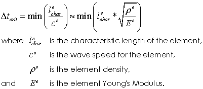
Initial mass scaling constant (Default: 1.0). The element density is evaluated using the grain density, fluid density, porosity and porous flow type (see Porous_flow_type on the Group data structure). The element density controls the critical time step for the geomechanical field ( Δtcrit) where
The geomechanical field is often solved using an explicit dynamic solution algorithm set up to provide approximately transient steady-state solutions. Transient steady-state can only be achieved if the inertia effects are negligible. This is generally achieved by: •selecting a time step close to the maximum allowable (e.g. Δt=fallowΔtcrit where fallow ≥ 0.25) •selecting the number of time steps to be large enough such that inertia effects are negligible by monitoring the dynamic effects using time history data; e.g. elastic and kinetic energy, nodal velocities, etc. Consequently mass-scaling is generally advantageous as it allows modifying the critical time step so that the desired number of time steps is achieved for a specified time. This time is generally dictated by the physics of the problem; e.g. the sedimentation rate. Mass-scaling modifies the density used in evaluation of the element mass used in the explicit dynamic solver without influencing any other operations that utilise density; e.g. gravity loading, etc. When mass-scaling is used the critical time step then becomes:
A mass-scale factor fmass > 1 therefore increases the critical time step by the square root of the mass-scaling factor, conversely a mass-scale factor fmass < 1 decreases the critical time step.
Notes •Initial_mass_scaling_constant can be used in conjunction with the globally applied mass-scaling specified using the Time_scaling_factors data structure •When using the explicit dynamics solver it is important that the element critical time step for all elements is similar. If any group of elements have values that are significantly higher than the majority of the domain this group will exhibit inertia effects which may degrade the solution. •If in Time_scaling_factors the Model_type is set to "Absolute_target" the mass-scaling constant is automatically evaluated and the Initial_mass_scaling_constant has no effect.
|
| Elastic_model_type Elastic model type |
Usage |
||||
|
||||
Description |
||||
Defines whether the elastic properties are isotropic or orthotropic. Valid states are: • 1 - "Isotropic" • 2 - "Transverse Isotropic" • 3 - "Orthotropic" • 4 - "Transverse Isotropic via Voight stiffness terms" • 5 - "Orthotropic via Voight stiffness terms"
Notes •If Elastic_model_type is not specified then by default: •The material is assumed to be orthotropic if Orthotropic_elastic_properties is specified with non-zero properties •The material is assumed to be isotropic if Orthotropic_elastic_properties is NOT specified with non-zero properties |
| Elastic_properties (or Isotropic_elastic_properties) Elastic properties (Geomechanical) |
Usage |
|||||||||||||||
|
|||||||||||||||
Description |
|||||||||||||||
The elastic properties are dependent on the model type:
Model 1 - Isotropic Elasticity The isotropic elastic properties comprise (2 values required): • Location 1 - "Young's Modulus" • Location 2 - "Poisson's Ratio"
Model 2 - Transverse Isotropic Elasticity The transverse elastic properties comprise: • Location 1 - "In plane Young's Modulus" • Location 2 - "Out of plane Young's Modulus" • Location 3 - "In plane Poisson's Ratio" • Location 4 - "Out of plane Poisson's Ratio" • Location 5 - "Out of plane Shear Modulus"
State Variables The input and output state variables are: •'Young11' - In plane Young's Modulus •'Young33' - Out of plane Young's Modulus •'Poiss12' - In plane Poisson's Ratio •'Poiss23' - Out of plane Poisson's Ratio •'Shear23' - Out of plane Shear Modulus
Model 3 - Orthotropic Elasticity The orthotropic elastic properties comprises: • Location 1 - "Young's Mod. in X" • Location 2 - "Young's Mod. in Y" • Location 3 - "Young's Mod. in Z" • Location 4 - "Poiss. Rat. XY plane" • Location 5 - "Poiss. Rat. YZ plane" • Location 6 - "Poiss. Rat. ZX plane" • Location 7 - "Shear Mod. XY plane" • Location 8 - "Shear Mod. YZ plane" • Location 9 - "Shear Mod. ZX plane"
State Variables The input and output state variables are: •'Young11' - Young's Mod. in X •'Young22' - Young's Mod. in Y •'Young33' - Young's Mod. in Z •'Poiss12' - Poiss. Rat. XY plane •'Poiss23' - Poiss. Rat. YZ plane •'Poiss31' - Poiss. Rat. ZX plane •'Shear12' - Shear Mod. XY plane •'Shear23' - Shear Mod. YZ plane •'Shear31' - Shear Mod. ZX plane
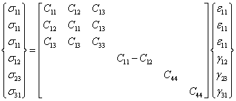
Model 4 - Transverse Isotropic Elasticity via Matrix Coefficients The transverse isotropic stiffness matrix may be defined in Voight notation as:
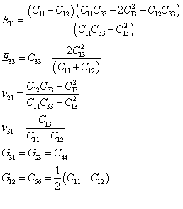
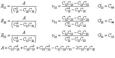
where the engineering parameters are defined from the stiffness terms via:
Model 4 allows these stiffness terms to be defined directly as: • Location 1 - "C11 stiffness term" • Location 2 - "C12 stiffness term" • Location 3 - "C13 stiffness term" • Location 4 - "C33 stiffness term" • Location 5 - "C44 stiffness term"
State Variables The input state variables are: •'C11' - C11 stiffness term •'C12' - C12 stiffness term •'C13' - C13 stiffness term •'C33' - C33 stiffness term •'C44' - C44 stiffness term
The output state variables are: •'Young11' - In plane Young's Modulus •'Young33' - Out of plane Young's Modulus •'Poiss12' - In plane Poisson's Ratio •'Poiss23' - Out of plane Poisson's Ratio •'Shear23' - Out of plane Shear Modulus
Notes •Model 4 is effectively the same as Model 2. The difference is the input data for Model 4 are the Cij variables. However, internally in the ParaGeo code, these variables are converted and expressed in the input variables for Model 2. Likewise for the output variables.
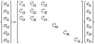
Model 5 - Orthotropic Elasticity via Matrix Coefficients The orthotropic stiffness matrix may be defined in Voight notation as:
where the engineering parameters are defined from the stiffness terms via:
Model 5 allows these stiffness terms to be defined directly as: • Location 1 - "C11 stiffness term" • Location 2 - "C12 stiffness term" • Location 3 - "C13 stiffness term" • Location 4 - "C22 stiffness term" • Location 5 - "C23 stiffness term" • Location 6 - "C33 stiffness term" • Location 7 - "C44 stiffness term" • Location 8 - "C55 stiffness term" • Location 9 - "C66 stiffness term"
State Variables The input state variables are: •'C11' - C11 stiffness term •'C12' - C12 stiffness term •'C13' - C13 stiffness term •'C22' - C22 stiffness term •'C23' - C23 stiffness term •'C33' - C33 stiffness term •'C44' - C44 stiffness term •'C55' - C55 stiffness term •'C66' - C66 stiffness term
The output state variables are: •'Young11' - Young's Mod. in X •'Young22' - Young's Mod. in Y •'Young33' - Young's Mod. in Z •'Poiss12' - Poiss. Rat. XY plane •'Poiss23' - Poiss. Rat. YZ plane •'Poiss31' - Poiss. Rat. ZX plane •'Shear12' - Shear Mod. XY plane •'Shear23' - Shear Mod. YZ plane •'Shear31' - Shear Mod. ZX plane
Notes •Model 5 is effectively the same as Model 3. The difference is the input data for Model 5 are the Cij variables. However, internally in the ParaGeo code, these variables are converted and expressed in the input variables for Model 3. Likewise for the output variables. •The transverse isotropic properties are defined in the element material coordinate system which is specified using the Coordinate_system data structure and assigned by the Material_coord_system keyword on the Groups data structure. •The orthotropic properties are defined in the element material coordinate system which is specified using the Coordinate_system data structure and assigned by the Material_coord_system keyword on the Groups data structure.
|
|||||||||||||||
| Elastic_properties_tvar Isotropic Elastic temperature variation (Geomechanical) |
Usage |
|||||||||||||||
|
|||||||||||||||
Description |
|||||||||||||||
The properties are dependent on the model type:
Model 1 - Isotropic Elasticity The isotropic elastic properties temperature variation comprise (2 values required): •Location 1 - Young's Modulus temperature variation •Location 2 - Poisson's Ratio temperature variation
Model 2 - Transverse Isotropic Elasticity The transverse isotropic elastic properties temperature variation comprise: •Location 1 - In-plane Young's modulus temperature variation •Location 2 - Out-of-plane Young's modulus temperature variation •Location 3 - In-plane Poisson's ratio temperature variation •Location 4 - Out-of-plane Poisson's ratio temperature variation •Location 5 - Out-of-plane Shear modulus temperature variation
Model 3 - Orthotropic Elasticity The Orthotropic elastic properties temperature variation comprise: •Location 1 - Young's Modulus in X direction temperature variation •Location 2 - Young's Modulus in Y direction temperature variation •Location 3 - Young's Modulus in Z direction temperature variation •Location 4 - Poisson's Ratio in X-Y plane temperature variation •Location 5 - Poisson's Ratio in Y-Z plane temperature variation •Location 6 - Poisson's Ratio in Z-X plane temperature variation •Location 7 - Shear Modulus in X-Y plane temperature variation •Location 8 - Shear Modulus in Y-Z plane temperature variation •Location 9 - Shear Modulus in Z-X plane temperature variation
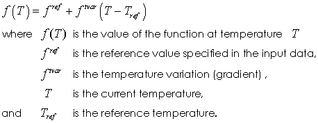
Notes •The temperature dependent elastic properties are evaluated using a function of the form:
|
|||||||||||||||
| Porous_elasticity_type Poroelastic type number |
Usage |
||||
|
||||
Description |
||||
Poroelastic type number. The models available comprise: • 1 - "CamClay Model" • 2 - "pc and p dependent Model" • 3 - "CamClay hysteresis unload." • 4 - "Rate dependent CamClay model" • 5 - "Cubic Nonlinear Elasticity" • 6 - "Rate dependent CamClay model"
|
| Porous_elastic_properties Porous elastic properties |
Usage |
|||||||||||||||
|
|||||||||||||||
Description |
|||||||||||||||
The porous elastic properties are model dependent.
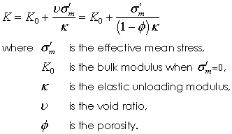
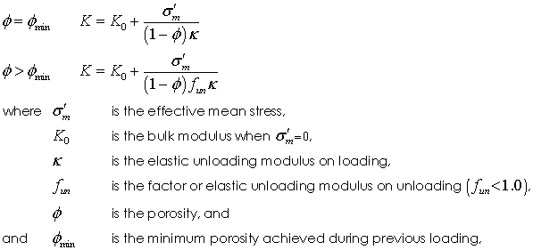
Model 1 - Cam Clay Model The Cam Clay poroelastic model defines the bulk modulus ( K) as:
While the model is commonly used in geomechanical simulations it suffers some drawbacks; i.e. •On unloading/reloading, which may occur during brittle faulting, the elasticity (stiffness) may become extremely low. •The elastic modulus is independent of the lithification process and therefore unsuitable forward modelling when diagenesis is considered.
The poroelastic parameters are: • Location 1 - "Reference Bulk modulus ( K0 )" • Location 2 - "Kappa (Unloading modulus) ( κ )" • Location 3 - "Minimum cutoff Young's modulus ( Emin) (Optional)" • Location 4 - "Maximum cutoff Young's modulus ( EMax) (Optional)"
If Emin and EMax are not specified then bounds are not applied to the evaluated young's Modulus.
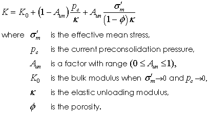
Model 2 - Porosity and Pressure Dependent Model The porosity and pore pressure dependent model defines the bulk modulus ( K) as:
For clarity the law is defined in terms of the pre consolidation pressure but the porosity dependence is due to the direct relationship between porosity and pre consolidation pressure. The law has the advantage that porosity reduction, due to either mechanical or diagenetic processes, results in an increase in bulk modulus that can only be removed by damaging the material sufficiently to return the porosity to its virgin state. Note that when ( Aun) = 1 then the law is identical to model 1 (Cam Clay)
The poroelastic parameters are: • Location 1 - "Reference Bulk modulus ( K0 )" • Location 2 - "Kappa (Unloading modulus) ( κ )" • Location 3 - "Porosity dependence factor ( Aun )" • Location 4 - "Minimum cutoff Young's modulus ( Emin) (Optional)" • Location 5 - "Maximum cutoff Young's modulus ( EMax) (Optional)"
If Emin and EMax are not specified then bounds are not applied to the evaluated young's Modulus.
Model 3 - Cam Clay model for hysteresis on unloading The Cam Clay poroelastic model defines the bulk modulus ( K) as: This is an augmented version of model 1 where the unloading modulus may be less than the loading modulus resulting reduced volume recovery on unloading; i.e.
The poroelastic parameters are: • Location 1 - "Reference Bulk modulus ( K0 )" • Location 2 - "Kappa (Unloading modulus) ( κ )" • Location 3 - "Unloading modulus factor ( fun )" • Location 4 - "Minimum cutoff Young's modulus ( Emin) (Optional)" • Location 5 - "Maximum cutoff Young's modulus ( EMax) (Optional)"
If Emin and EMax are not specified then bounds are not applied to the evaluated young's Modulus.
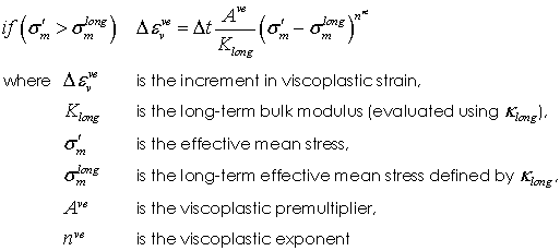
Model 4 - Rate dependent Cam Clay Model This model is a rate dependent version of the cam clay model where the poroelastic response is time dependent and defined by short-term unloading modulus ( κshort) and a long-term unloading modulus ( κlong ), where κshort < κlong. The short-term response is therefore stiffer, and rate dependent creep, defined via rate dependent parameters (premultiplier ( A) and exponent ( n )), results in relaxation to the long-term response. The creep law is defined as:
The poroelastic parameters are: • Location 1 - "Reference Bulk modulus ( K0 )" • Location 2 - "Long term Kappa (Unloading modulus) ( κlong )" • Location 3 - "Short term Kappa (Unloading modulus) ( κshort )" • Location 4 - "Pre multiplier" ( A )" • Location 5 - "Exponent ( n )" • Location 6 - "Minimum cutoff Young's modulus ( Emin) (Optional)" • Location 7 - "Maximum cutoff Young's modulus ( EMax) (Optional)"
If Emin and EMax are not specified then bounds are not applied to the evaluated young's Modulus.
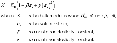
Model 5 - Cubic Nonlinear Elasticity This model is a rate independent nonlinear elasticity law defined as:
The poroelastic parameters are: • Location 1 - "Reference Bulk modulus ( K0 )" • Location 2 - "Beta constant" • Location 3 - "Gamma constant" • Location 4 - "Minimum cutoff Young's modulus ( Emin) (Optional)" • Location 5 - "Maximum cutoff Young's modulus ( EMax) (Optional)"
If Emin and EMax are not specified then bounds are not applied to the evaluated young's Modulus.
Model 6 - Rate dependent Cam Clay Model Principal Stress Based Flow Rul This model is a rate dependent version of the cam clay model where the poroelastic response is time dependent and defined by short-term unloading modulus ( κshort) and a long-term unloading modulus ( κlong ), where κshort < κlong. The short-term response is therefore stiffer, and rate dependent creep, defined via rate dependent parameters (premultiplier ( A) and exponent ( n )), results in relaxation to the long-term response. The creep law is defined as:
The poroelastic parameters are: • Location 1 - "Reference Bulk modulus ( K0 )" • Location 2 - "Long term Kappa (Unloading modulus) ( κlong )" • Location 3 - "Short term Kappa (Unloading modulus) ( κshort )" • Location 4 - "Pre multiplier" ( A )" • Location 5 - "Exponent ( n )" • Location 6 - "Compaction direction factor varying from hydrostatic to uniaxial compaction" • Location 7 - "Minimum cutoff Young's modulus ( Emin) (Optional)" • Location 8 - "Maximum cutoff Young's modulus ( EMax) (Optional)"
Notes •Compaction direction factor defines whether if the compaction is predominantly hydrostatic porosity reduction or uniaxial porosity loss. The factor has a range ( fflow) where ( 0.0 ≤ fflow ≤ 1.0) and 1.0 corresponds to hydrostatic compaction and 0.0 corresponds to uniaxial compaction.
If Emin and EMax are not specified then bounds are not applied to the evaluated young's Modulus.
|
|||||||||||||||
| Shear_modulus fixed shear modulus for poroelastic material |
Usage |
||||
|
||||
Description |
||||
Defines a fixed shear modulus value for a poroelastic material (variable Poisson's ratio).
|
| Hysteresis_elasticity_type Poroelastic type number |
Usage |
||||
|
||||
Description |
||||
Hysteresis type number. One model is currently available:
• 1 - "Two parameter model"
|
| Hysteresis_elastic_properties Porous elastic properties |
Usage |
|||||||||||||||
|
|||||||||||||||
Description |
|||||||||||||||
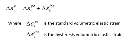
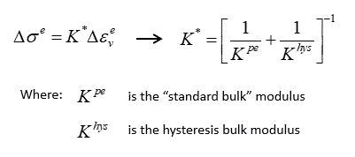
Hysteresis elastic models impose hysteresis on any poroelastic model by decomposing the elastic strain into standard and hysteresis components; i.e.
The combined bulk modulus ( K*) is then defined as:
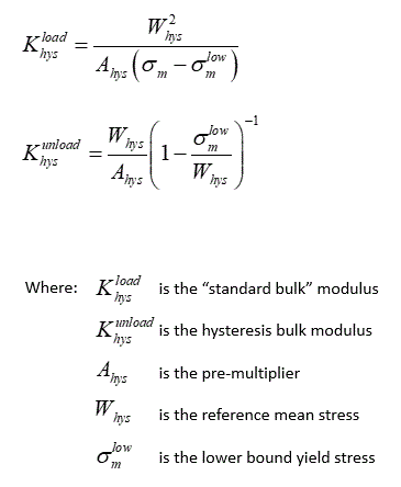
Model 1 - Two parameter model This model defines the loading and unloading hysteresis bulk modulii as;
The hysteresis parameters are: • Location 1 - "Pre multiplier ( Ahys )" • Location 2 - "Reference mean stress ( Whys )"
|
|||||||||||||||
| Total_strain_flag Use total strain for elasticity update |
Usage |
||||
|
||||
Description |
||||
Defines whether the elastic stress is updated incrementally or using total strain. Incremental update is default but total strain update is required for elastic damage models or temperature dependent elasticity. • 0 - "Incremental update (default)" • 1 - "Total strain update"
|
| Porous_elasticity_update_type Porous elasticity update type number |
Usage |
||||
|
||||
Description |
||||
Porous elasticity update type number. Two models are available:
• 1 - "Secant method" • 2 - "Fixed iteration step"
|
| Porosity_model_type Porosity Type (Optional) |
Usage |
||||
|
||||
Description |
||||
Three porosity models are available: • 1 - "Constant Porosity (defaults to model 2 if the geomechanical field is active)" • 2 - "Porosity updated due to geomechanical deformation (Default)" • 3 - "Porosity dependent on pore pressure (Generally only used in single field porous flow analysis where geomechanical deformation is not computed."
|
| Porosity Porosity (Compulsory if porous material) |
Usage |
||||
|
||||
Description |
||||
Porosity of the material. If a porosity dependent constitutive model (e.g. SR4 plasticity model) is used this porosity must be the porosity corresponding to the reference pre consolidation pressure ( pc0 ). If the initial porosity differs from this reference porosity it may be defined using either the Geostatic_initial_conditions or Group_initial_conditions data structure.
|
| Porosity_vs_pressure Porosity vs. pore pressure curve (Optional) |
Usage |
|||||||||||||||
|
|||||||||||||||
Description |
|||||||||||||||
Porosity vs. pore pressure curve. The data is provided as a 2-D table where: •Location 1 - "Pore press." - "List of pore pressure values" •Location 2 - "Porosity" - "Porosity for each pressure specified in Row 1"
|
|||||||||||||||
| Tortuosity_model_type Tortuosity Type (Gas flow Only) |
Usage |
||||
|
||||
Description |
||||
Tortuosity is required for evaluation of the Knudsen number in gas flow problems with Knudsen diffusion. Two types of Tortuosity model are available: • 1 - "Constant tortuosity" • 2 - "Pressure dependent tortuosity"
|
| Tortuosity Tortuosity (Gas flow Only) |
Usage |
||||
|
||||
Description |
||||
Tortuosity for the constant tortuosity model.
|
| Tortuosity_vs_pressure Tortuosity vs. pore pressure curve |
Usage |
|||||||||||||||
|
|||||||||||||||
Description |
|||||||||||||||
•"Pore press." •"Tortuosity" Tortuosity vs. pore pressure curve. The data is provided as a 2-D table where: •Location 1 - "list of pore pressures values" •Location 2 - "Tortuosity for each specified pressure value"
|
|||||||||||||||
| Plastic_material_type Plasticity type number |
Usage |
||||
|
||||
Description |
||||
Defines the elastoplastic model to be used. Models available are: • 1 - "SR3 pressure dependent plasticity model" • 2 - "SR4 pressure dependent plasticity model" • 4 - "Isotropic Modified Cam-Clay model" • 5 - "Drucker Prager model (modified)" • 51 - "Stress-based Rotating Crack model" • 6 - "Strain-based Rotating Crack model" • 7 - "von Mises model" • 8 - "Hill anisotropic model"
|
| Plastic_properties Plastic properties |
Usage |
|||||||||||||||
|
|||||||||||||||
Description |
|||||||||||||||
The plastic properties are model dependent and are defined as:
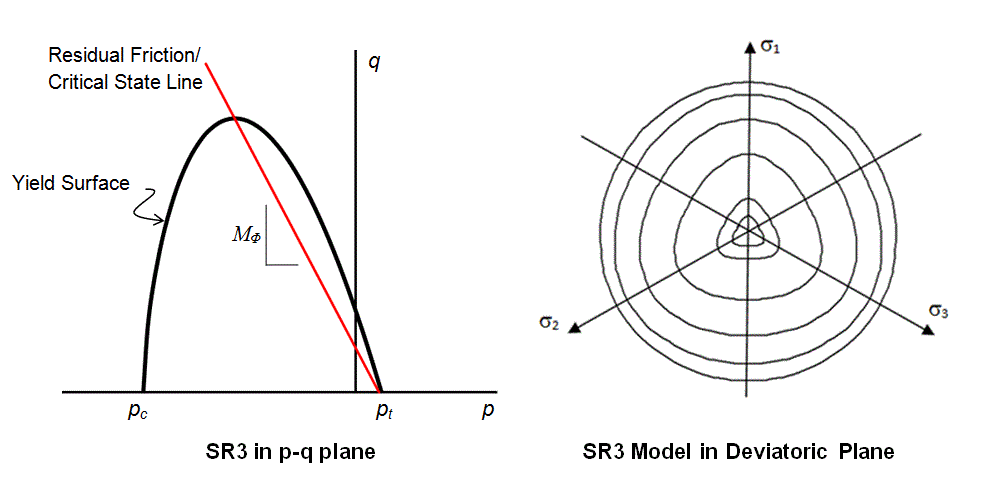
Model 1 - SR3 Plasticity Model The state boundary surface for the SR3 model is a smooth invariant surface that intersects the hydrostatic axis in both tension and compression (Crook et al., 2006). The yield surface is smooth in the deviatoric plane with the state boundary surface being defined using a deviatoric correction term, whereas the flow potential is circular.
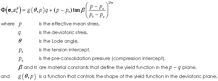
Yield Surface Definition in the p-q Plane The yield surface is defined as:
Yield Surface Definition in the Deviatoric Plane In the deviatoric plane the yield surface is defined as:
Potential Surface Definition The potential surface is defined as:
Material Properties • Location 1 - Tension intercept ( pt) • Location 2 - Initial pre consolidation pressure ( pc) • Location 3 - Friction parameter ( β) • Location 4 - Dilation parameter ( ψ) • Location 5 - Deviatoric plane parameter ( β0) (Generally 0.6) • Location 6 - Deviatoric plane parameter ( β1) (Generally 0.6) • Location 7 - Deviatoric plane parameter ( α) (Generally 0.25) • Location 8 - Yield surface Exponent ( n)
State Variables The default output state variables for the SR3 Model are: •'P_strn ' - Plastic Strain •'P_strn_r' - Plastic Strain Rate •'P_strnv ' - Plastic Volume Strain •'P_comc ' - Pre-Consolidation Pressure •'P_tenc ' - Tensile Intercept •'P_beta' - Friction parameter ( β) •'P_phi' - Dilation parameter ( ψ) •'P_expn' - Yield surface Exponent ( n)
Additional state variables that may be requested (see Output_data ) are: •'P_strnxx' - Plastic Strain Component XX •'P_strnyy' - Plastic Strain Component YY •'P_strnzz' - Plastic Strain Component ZZ •'P_strnxy' - Plastic Strain Component XY •'P_strnyz' - Plastic Strain Component YZ •'P_strnzx' - Plastic Strain Component ZX •'P_conver' - Convergence flag •'P_flag ' - Plastic flag marking all elements that are plastic in this step •'P_state ' - Plastic state •'P_stten ' - Plastic state Tension (all elements that at some stage yielded in tension) •'P_stshr ' - Plastic State Shear (all elements that at some stage yielded in shear) •'P_stcap ' - Plastic State Cap (all elements that at some stage yielded in compression)
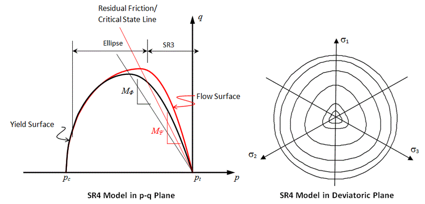
Model 2 - SR4 Plasticity Model The state boundary surface for the SR4 model is described by a smooth three-invariant surface composed of two functions that intersect in a continuous manner at the point of maximum deviatoric stress. The shear side is defined using the SR3 surface (Crook et al., 2006) and the compression side is defined by an ellipse; i.e. in a similar manner as the standard Cam Clay model (Wood, 1990). The flow potential surface is the same form as the state boundary surface but is defined with two different parameters. This enables the residual friction (critical state) line to be defined to intersect the state boundary surface on the shear side, as opposed to at the location of the peak stress. This is consistent with experimental observations on sands and clays (e.g. Wood, 1990). Both surfaces are smooth in the deviatoric plane with the state boundary surface being defined using a deviatoric correction term, whereas the flow potential is circular.
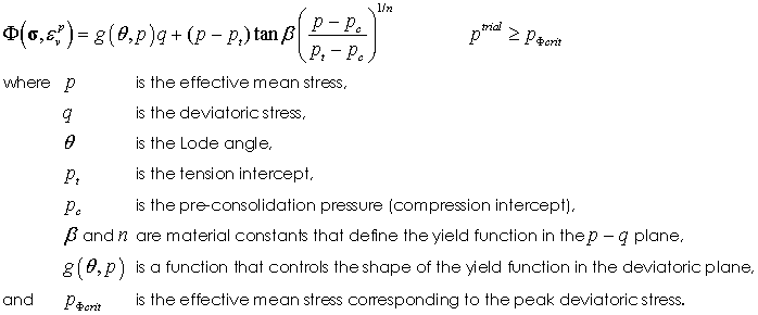
Yield Surface Definition in the p-q Plane The shear side of the yield surface is defined as:
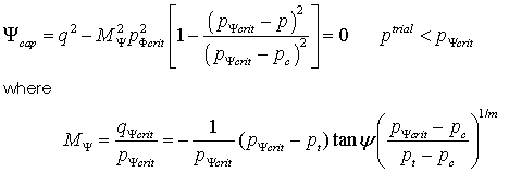
The compression side of the yield surface is defined as:
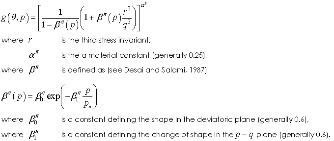
Yield Surface Definition in the Deviatoric Plane In the deviatoric plane the yield surface is defined as:
Potential Surface Definition The shear side of the potential surface is defined as:
The compression side of the potential surface is defined as:
Material Properties • Location 1 - Tension intercept ( pt) • Location 2 - Initial pre consolidation pressure ( pc) • Location 3 - Friction parameter ( β) • Location 4 - Dilation parameter ( ψ) • Location 5 - Deviatoric plane parameter ( β0) (Generally 0.6) • Location 6 - Deviatoric plane parameter ( β1) (Generally 0.6) • Location 7 - Deviatoric plane parameter ( α) (Generally 0.25) • Location 8 - Yield surface Exponent ( n) • Location 9 - Flow potential surface Exponent ( m)
State Variables The default output state variables for the SR4 Model are: •'P_strn' - Plastic Strain •'P_strn_r' - Plastic Strain Rate •'P_strnv' - Plastic Volume Strain •'P_comc' - Pre-Consolidation Pressure •'P_tenc' - Tensile Intercept •'P_beta' - Friction parameter ( β) •'P_phi' - Dilation parameter ( ψ) •'P_expn' - Yield surface Exponent ( n) •'P_expm' - Flow potential surface Exponent ( m)
Additional state variables that may be requested (see Output_data ) are: •'P_strnxx' - Plastic Strain Component XX •'P_strnyy' - Plastic Strain Component YY •'P_strnzz' - Plastic Strain Component ZZ •'P_strnxy' - Plastic Strain Component XY •'P_strnyz' - Plastic Strain Component YZ •'P_strnzx' - Plastic Strain Component ZX •'P_conver' - Convergence flag •'P_flag ' - Plastic flag marking all elements that are plastic in this step •'P_state ' - Plastic state •'P_stten ' - Plastic state Tension (all elements that at some stage yielded in tension) •'P_stshr ' - Plastic State Shear (all elements that at some stage yielded in shear) •'P_stcap ' - Plastic State Cap (all elements that at some stage yielded in compression)
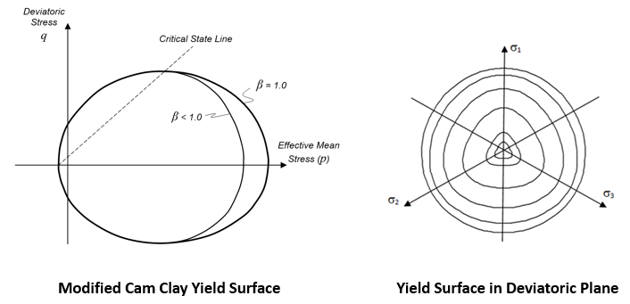
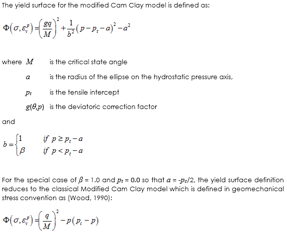
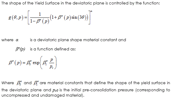
Model 4 - Isotropic Modified Cam-Clay Model The modified Cam Clay yield surface is an extension of the classical modified Cam Clay model (Wood, 1990). The Cam Clay model is based on critical state soil mechanics and describes the evolution of the yield surface in terms of the change in void ratio or porosity. The basic shape of the yield surface is elliptical, but in the modified form in ParaGeo the shape of the Cap may be modified by using an additional parameter (β). Additionally: •The yield surface is offset in the p-q plane by specification of a tensile intercept (pt) •A deviatoric correction term g(θ,p) is used to modify the shape of the yield surface in the deviatoric plane
Yield Surface
Yield Surface in the Deviatoric Plane
Material Properties • Location 1 - Tension intercept ( pt) • Location 2 - Initial pre consolidation pressure ( pc) • Location 3 - Constant beta ( β) • Location 4 - Constant M ( M)
State Variables The default output state variables for the Isotropic Modified Cam-Clay Model are: •'P_strn ' - Plastic Strain •'P_strn_r' - Plastic Strain Rate •'P_strnv ' - Plastic Volume Strain •'P_comc ' - Pre-Consolidation Pressure •'P_tenc ' - Tensile Intercept
Additional state variables that may be requested (see Output_data ) are: •'P_strnxx' - Plastic Strain Component XX •'P_strnyy' - Plastic Strain Component YY •'P_strnzz' - Plastic Strain Component ZZ •'P_strnxy' - Plastic Strain Component XY •'P_strnyz' - Plastic Strain Component YZ •'P_strnzx' - Plastic Strain Component ZX •'P_conver' - Convergence flag •'P_flag ' - Plastic flag marking all elements that are plastic in this step •'P_state ' - Plastic state •'P_epvcom' - Most compressive volumetric plastic strain •'P_epvten' - Most tensile volumetric plastic strain
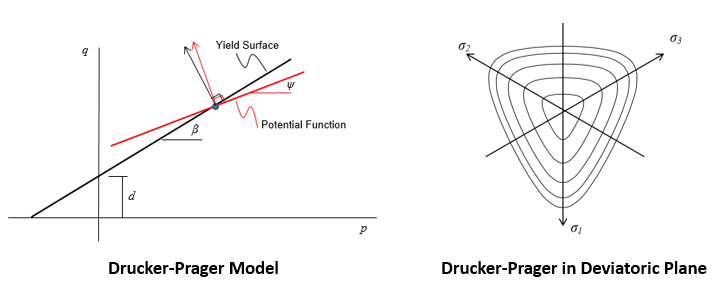
Model 5 - Drucker Prager Model The Drucker-Prager model is a shear yield surface that is most suitable for representation of brittle materials where yielding/failure is predominantly in shear (i.e when mechanical compaction can be neglected).
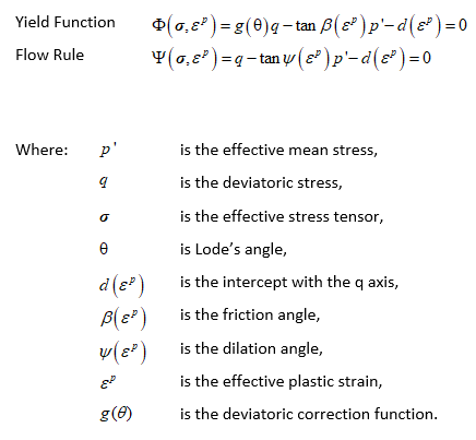
Yield and Flow surfaces The Yield and Flow surfaces are defined as:
Note that d, β and ψ are defined as a function of plastic strain and the function must be defined in a tabular form using the keyword Hardening_properties.
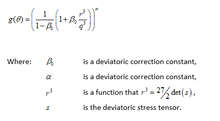
The deviatoric correction term is defined as:
Material Properties • Location 1 - Intercept d ( d) • Location 2 - Friction angle ( β) in Degrees • Location 3 - Dilation angle ( ψ) in Degrees • Location 4 - Beta0 (deviatoric plane) ( β0) • Location 5 - Alpha (deviatoric plane) ( α)
State Variables The default output state variables for the Drucker Prager Model are: •'P_strn ' - Plastic Strain •'P_strn_r' - Plastic Strain Rate •'P_strnv ' - Plastic Volume Strain •'P_d ' - Intercept, d •'P_beta ' - Friction angle, beta •'P_psi ' - Dilation angle, psi
Additional state variables that may be requested (see Output_data ) are: •'P_strnxx' - Plastic Strain Component XX •'P_strnyy' - Plastic Strain Component YY •'P_strnzz' - Plastic Strain Component ZZ •'P_strnxy' - Plastic Strain Component XY •'P_strnyz' - Plastic Strain Component YZ •'P_strnzx' - Plastic Strain Component ZX •'P_conver' - Convergence flag •'P_flag ' - Plastic flag marking all elements that are plastic in this step •'P_state ' - Plastic state
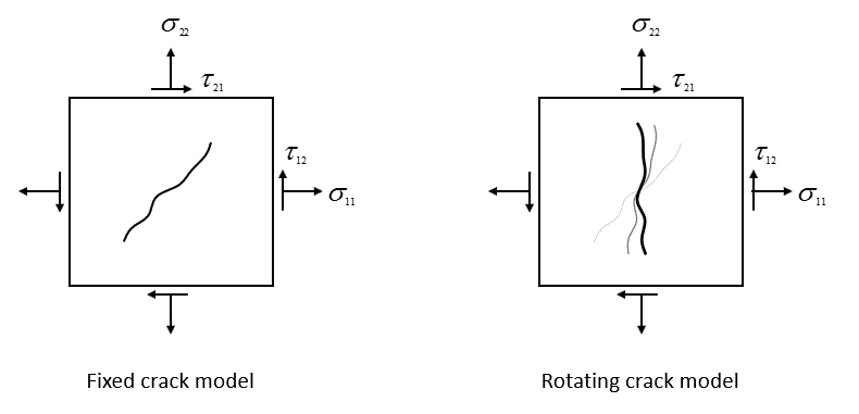
Model 51 - Rotating Cracking Model (Stress based) The rotating crack model 51 is a tensile strength stress-based model derived from the Rankine failure criterion by which a fracture normal to the most tensile stress is developed if the tensile stress exceeds the tensile strength. As opposed to the fixed crack model, the direction of the propagating fracture rotates along with the principal stresses so that the fracture plane is always normal to the current direction of the most tensile stress. This model was originally developed to capture the post-fracture behaviour of reinforced concrete structures to simulate the partial closure of existing microcracks and formation of a new system of microcracks consistent with the new principal stress orientation. This model is available for both 2D and 3D simulations (as opposed to the strain-based rotating crack which is only available for 2D).
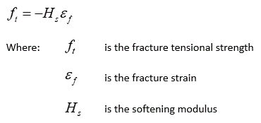
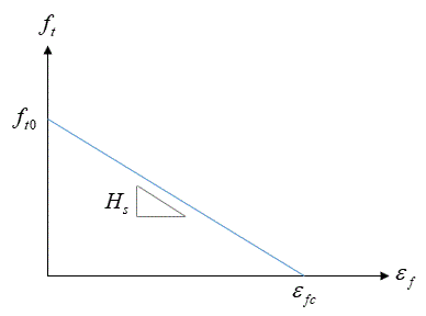
When the tensile fracture strength is exceeded the fracture strength decreases with the ongoing fracture strain as defined by the softening law. Assuming linearity in the variation of fracture strength with fracture strain then the softening law is formulated as:
When the fracture strain reaches the critical value
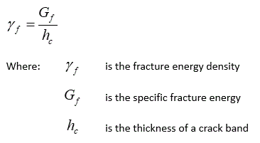
The area under the softening plot is defined as the fracture energy density which is expressed as:
Because of the considered linearity of the softening behaviour the softening slope may be determined from the fracture properties of the material as:
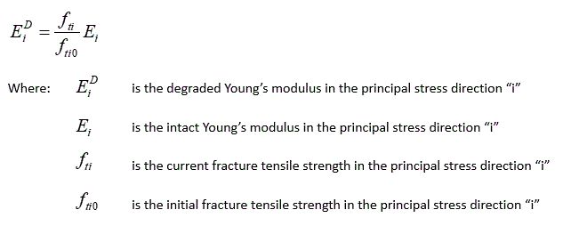
The model considers local degradation of elastic properties (Young's modulus and Poisson's ratio) as tensile strength reduces with softening. The degraded Young's modulus is defined as:
Material Properties Only the 2 first material properties listed below are compulsory (defining IDM =2) while the 3rd one is optional: • Location 1 - Tensile Strength ( Ft) • Location 2 - Fracture energy ( Gf) • Location 3 - Shear retention factor ( β) which defines the shear transfer across a crack and has a value between 0 (no transfer) and 1 (stress locking) Default value is 0.1
State Variables The default output state variables for the Stress-based Rotating Cracking Model are: •'R_state1' - Fracture state in first principal stress direction •'R_ft1' - Tensile stress in first principal stress direction •'R_psang1' - Principal stress angle 11 (Not crack angle) •'R_strn1' - Fracture strain in first principal direction •'R_strs1' - Fracture stress in first principal direction •'R_edamg1' - Damaged elastic modulus in first principal stress direction •'R_esoft1' - Softening slope •'R_epstn1' - Total strain in first principal stress direction •'R_damfac' - Damage factor
Model 6 - Rotating Cracking Model (Strain based) The rotating crack model 6 is a tensile strength strain-based model derived from the Rankine failure criterion by which a fracture normal to the most tensile stress is developed if the tensile stress exceeds the tensile strength. As opposed to the fixed crack model, the direction of the propagating fracture rotates along with the principal stresses so that the fracture plane is always normal to the current direction of the most tensile stress. This model was originally developed to capture the post-fracture behaviour of reinforced concrete structures to simulate the partial closure of existing microcracks and formation of a new system of microcracks consistent with the new principal stress orientation. The model is currently only applicable in 2D simulations.
When the tensile fracture strength is exceeded the fracture strength decreases with the ongoing fracture strain as defined by the softening law. Assuming linearity in the variation of fracture strength with fracture strain then the softening law is formulated as:
When the fracture strain reaches the critical value
The area under the softening plot is defined as the fracture energy density which is expressed as:
Because of the considered linearity of the softening behaviour the softening slope may be determined from the fracture properties of the material as:
The model considers local degradation of elastic properties (Young's modulus and Poisson's ratio) as tensile strength reduces with softening. The degraded Young's modulus is defined as:
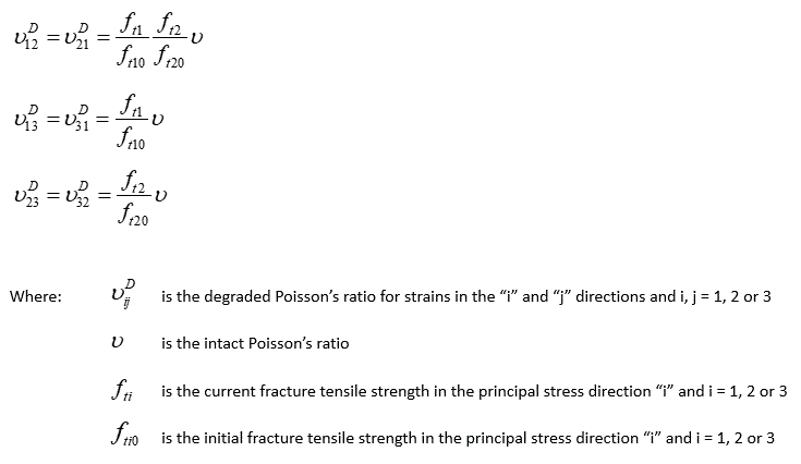
And the degraded Poisson's ratio is given by (assuming 2D and no degradation of tensile strength in the out-of-plane direction):
Material Properties • Location 1 - Tensile Strength ( Ft) • Location 2 - Fracture energy ( Gf) • Location 3 - Shear retention factor ( β) which defines the shear transfer across a crack and has a value between 0 (no transfer) and 1 (stress locking)
State Variables The default output state variables for the Strain-based Rotating Cracking Model are: •'R_ft1 ' - Tensile stress in first principal stress direction •'R_ft2 ' - Tensile stress in second principal stress direction •'R_ft3 ' - Tensile stress in third principal stress direction •'R_epstn1' - Total strain in first principal stress direction •'R_epstn2' - Total strain in second principal stress direction •'R_epstn3' - Total strain in third principal stress direction •'R_edamg1' - Damaged elastic modulus in first principal stress direction •'R_edamg2' - Damaged elastic modulus in second principal stress direction •'R_edamg3' - Damaged elastic modulus in third principal stress direction •'R_damfac' - Damage factor •'R_state1' - Fracture state in first principal stress direction •'R_state2' - Fracture state in second principal stress direction •'R_state3' - Fracture state in third principal stress direction •'R_strn1 ' - Fracture strain in first principal direction •'R_strn2 ' - Fracture strain in second principal direction •'R_strn3 ' - Fracture strain in third principal direction •'R_strs1 ' - Fracture stress in first principal direction •'R_strs2 ' - Fracture stress in second principal direction •'R_strs3 ' - Fracture stress in third principal direction Additional state variables that may be requested (see Output_data ) are: •'P_flag ' - Yielding flag •'R_psang1' - Principal stress angle 11 (Not crack angle) •'R_psang2' - Principal stress angle 22 (Not crack angle) •'R_psang3' - Principal stress angle 33 (Not crack angle)
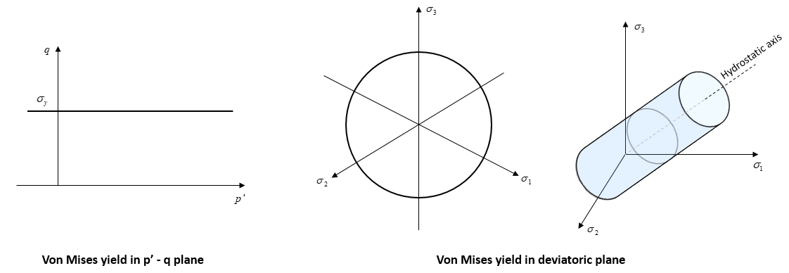
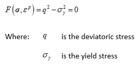
Model 7 - von Mises Model The von Mises model is a shear yield surface is independent of the effective mean stress and is suitable for metals
Yield and Flow surfaces The Yield and Flow surfaces are defined as:
Material Properties • Location 1 - Yield stress ( σy)
Generally a hardening curve is used, defined by hardening type 7, to provide the relationship between yield strength and effective plastic strain
State Variables The default output state variables for the Von Mises Model are: •'P_strn ' - Plastic Strain •'P_strn_r' - Plastic Strain Rate •'P_yield ' - Current yield stress
Additional state variables that may be requested (see Output_data ) are: •'P_strnxx' - Plastic Strain Component XX •'P_strnyy' - Plastic Strain Component YY •'P_strnzz' - Plastic Strain Component ZZ •'P_strnxy' - Plastic Strain Component XY •'P_strnyz' - Plastic Strain Component YZ •'P_strnzx' - Plastic Strain Component ZX •'P_flag ' - Plastic flag marking all elements that are plastic in this step
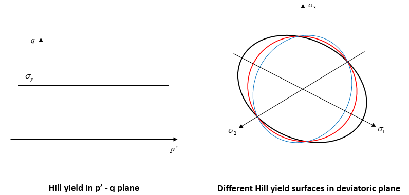
Model 8 - Hill Anisotropic Model The hill model is an anisotropic extension of the von Mises yield surface and is independent of the effective mean stress and is suitable for metals
Yield and Flow surfaces The Yield and Flow surfaces are defined as:
Material Properties • Location 1 - Yield stress ( σy)
Note that in order to define Hill anisotropy Plastic_anisotropic_type and Plastic_anisotropic_properties must be specified.
Generally a hardening curve is used, defined by hardening type 7, to provide the relationship between yield strength and effective plastic strain
State Variables The default output state variables for the Drucker Prager Model are: •'P_strn ' - Plastic Strain •'P_strn_r' - Plastic Strain Rate •'P_yield ' - Current yield stress
Additional state variables that may be requested (see Output_data ) are: •'P_strnxx' - Plastic Strain Component XX •'P_strnyy' - Plastic Strain Component YY •'P_strnzz' - Plastic Strain Component ZZ •'P_strnxy' - Plastic Strain Component XY •'P_strnyz' - Plastic Strain Component YZ •'P_strnzx' - Plastic Strain Component ZX •'P_flag ' - Plastic flag marking all elements that are plastic in this step
|
|||||||||||||||
| Hardening_type Hardening type number |
Usage |
||||
|
||||
Description |
||||
The Hardening type number is dependent on the material model. Valid values are:
• 1 - User defined Cam Clay: A piecewise linear curve derived directly from the analytical curve predicted by the standard Cam Clay ( k - l) model expressed as tabular data (Default) • 2 - User defined Cam-Clay: A smoothed piecewise linear curve derived directly from the analytical curve predicted by the standard Cam-Clay ( k - l) model expressed as tabular data. Defined via a constrained b-spline (more expensive and only required if the softening slope is very steep and convergence problems are encountered) • 3 - Analytical Cam Clay hardening • 8 - Analytical Cam Clay formulated as function of total plastic volume strain (suitable for temperature dependent hardening) • 6 - A piecewise linear curve to define the variation of the cohesion intercept ( d ), the friction angle ( β) (Degrees) and the dilation angle ( ψ) (Degrees) as a function of the effective plastic strain ( εp ). • 7 - A piecewise linear curve to define the variation of the yield strength ( σy) as a function of the effective plastic strain ( εp ).
|
| Hardening_properties Hardening properties for plasticity models |
Usage |
|||||||||||||||
|
|||||||||||||||
Description |
|||||||||||||||
The hardening data is dependent on the model type
Models 1 and 2 - SR3 and SR4 Tabular Data Hardening properties for SR3 and SR4 plasticity models. The data is provided as a 2-D table where: • Location 1 - list of volumetric plastic strains • Location 2 - pre consolidation pressure ( pc) for each volumetric plastic strain specified in Row 1 • Location 3 - tension intercept ( pt) for each volumetric plastic strain specified in Row 1
• Location 1 - list of volumetric plastic strains • Location 2 - pre consolidation pressure ( pc) for each volumetric plastic strain specified in Row 1 • Location 3 - tension intercept ( pt) for each volumetric plastic strain specified in Row 1
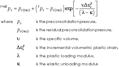
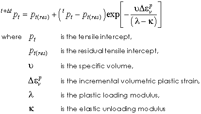
Model 3 - Cam Clay Analytical Model Data This model is a cam clay type hardening model based on the incremental volumetric plastic strain. It is defined as
Hardening properties for analytical Cam Clay model is: • Location 1 - Loading/unloading modulus ( k) - not used if poroelasticity specified • Location 2 - Consolidation modulus ( l) • Location 3 - pc(res) Residual value of pre consolidation pressure ( pc) • Location 4 - pt(res) Residual value of the tension intercept ( pt)
Note that pc(res) and pt(res) take default values of 0.01* pc and pt respectively if not defined.
Model 6 - Drucker Prager Model Tabular Data Hardening properties for plasticity models. The data is provided as a 2-D table where: • Location 1 - Effective plastic strain ( εp) • Location 2 - Intercept d ( d) • Location 3 - Friction angle ( β) (Degrees) • Location 4 - Dilation angle ( ψ) (Degrees)
Model 7 - von Mises Mises Tabular Data Hardening properties for plasticity models. The data is provided as a 2-D table where: • Location 1 - Effective plastic strain ( εp) • Location 2 - Yield strength ( σy)
Notes •Hardening model 7 is applicable to the von Mises and Hill material models
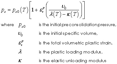
Model 8 - Cam Clay Analytical Model (total volumetric plastic strain) This model is a cam clay type hardening model where the evolution of pc is based on the total volumetric plastic strain. It is defined as
The evolution of pt is defined in the same manner as hardening model 3; i.e.
As it is defined using the initial value of pc0 it is suitable for defining temperature dependent hardening laws where pc0, λ and κ are temperature dependent. The hardening properties are: Hardening properties for analytical Cam Clay model is:
• Location 1 - Loading/unloading modulus ( k) - not used if poroelasticity specified • Location 2 - Consolidation modulus ( l)
Notes •Hardening model 8 is only applicable to the SR4 material model
|
|||||||||||||||
| Hardening2_update_frequency Hardening variable time/temperature table update interval |
Usage |
||||
|
||||
Description |
||||
Frequency for updating the hardening properties (default =100 steps for explicit solution and =1 for implicit solution). Values are interpolated between the hardening property data in the table.
Notes •For explicit solution of the mechanical field in non-coupled analysis the recommended update frequency is Hardening2_update_frequency > = 100 •For thermal, flow and coupled analysis the recommended update frequency is Hardening2_update_frequency = 1 |
| Hardening_variable2_name Hardening variable2 name |
Usage |
||||
|
||||
Description |
||||
Defines the variable upon which hardening is depending. Valid options are: • 1 - Allows to define a hardening table which varies as a function of time • 2 - Allows to define a hardening table which varies as a function of temperature
|
| Hardening_variable2_values List of Hardening variable2 values |
Usage |
|||||||||||||||
|
|||||||||||||||
Description |
|||||||||||||||
List of Hardening variable2 values.
|
|||||||||||||||
| Hardening_properties2 Hardening properties2 TABLE |
Usage |
|||||||||||||||
|
|||||||||||||||
Description |
|||||||||||||||
The data is provided as a 3-D table where a hardening table is defined for each time point. Note that there must be a minimum of two sets of hardening properties in the table.
|
|||||||||||||||
| Plastic_anisotropic_type Plastic anisotropy type number |
Usage |
||||
|
||||
Description |
||||
Anisotropy of the yield surface is defined by:
where ( σy) is the yield stress and the standard definition of deviatoric stress ( q) is replaced by an equivalent anisotropic definition ( qorth) defined via:
where
and the stresses in the local material coordinate system are defined as:
Crook et al. (2002) presented an orthotropic Cam Clay model specifically developed for representation of laminated shales. Shale may be described as a transverse isotropic material and experimental studies (Niandou et al., 1997) have shown that:
•The variation of compressive strength with the angle between the bedding planes and loading direction is such that the maximum compressive strength occurs when the loading direction is either parallel or perpendicular to the bedding planes. •The minimum compressive stress occurs when the loading to bedding plane orientation lies between 30º and 60º where the high shear stresses promote failure on the bedding planes.
Using the notation of Hashagen and de Borst (2001) for the general orthotropic case (Anisotropic model 1)
and
Anisotropy Models Three anisotropy definitions may be used with the plasticity models: • 1 - Transverse Isotropic (Constant anisotropy) • 2 - Orthotropic (Constant anisotropy) • 3 - Rotational Hardening (Constant anisotropy)
|
| Plastic_anisotropic_properties Plastic anisotropy properties |
Usage |
|||||||||||||||
|
|||||||||||||||
Description |
|||||||||||||||
The plastic anisotropy properties are model dependent and are defined as:
Model 1 - Transverse Isotropic (Constant anisotropy) The transverse isotropic q matrix is defined as
and
And the model is therefore defined via three parameters: • Location 1 - alpha 4 ( α4) • Location 2 - alpha 5 ( α5) • Location 3 - alpha 8 ( α8)
Model 2 - Orthotropic (Constant anisotropy) The anisotropic q matrix is defined via six parameters: • Location 1 - alpha 4 ( α4) • Location 2 - alpha 5 ( α5) • Location 3 - alpha 6 ( α6) • Location 4 - alpha 7 ( α7) • Location 5 - alpha 8 ( α8) • Location 6 - alpha 9 ( α9)
Model 3 - Rotational Hardening (Constant anisotropy) The anisotropic q matrix is defined via one parameter: • Location 1 - alpha (( α)
|
|||||||||||||||
| Rate_dependent_type The Strain rate dependent SR3 model number |
Usage |
||||
|
||||
Description |
||||
Two Strain rate dependent SR3 model are implemented. Valid values are: • 1 - Simple power law; • 2 - Power Law with Accelerated Creep at High Deviatoric Stress
|
| Rate_dependent_properties Rate dependent Properties |
Usage |
|||||||||||||||
|
|||||||||||||||
Description |
|||||||||||||||
The Strain rate dependent SR3 model properties are defined as:
Model 1 - Simple power law
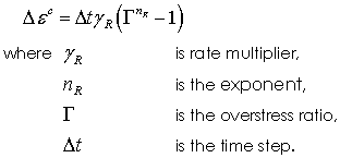
In the power law model the variable Gamma which defines the ratio between the two surfaces is related to the creep strain by the following function:
The input prroperties are then: • Location 1 - GammaR (Rate multiplier) • Location 2 - Exponent nR
Model 2 - Power Law with Accelerated Creep at High Deviatoric Stress
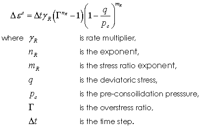
In the power law model with accelerated creep at high deviatoric stress (q) the variable Gamma which defines the ratio between the two surfaces is related to the creep strain by the following function:
The input properties are then: • Location 1 - GammaR (Rate multiplier) • Location 2 - Exponent nR • Location 3 - Exponent mR controlling acceleration for high q
|
|||||||||||||||
| Subloading_surface_type Subloading surface models |
Usage |
||||
|
||||
Description |
||||
Subloading_surface_type keyword may be added to a material defined with SR3 plasticity to consider a double surface sub-loading model. This enables to account for non-linear pre-yield behaviour. The input value defines the model to be used for the sub-loading surface. The available models are: • 1 - Log rate with hardening/softening threshold, which is designed to enable representation of pre peak stress path nonlinearity in current day material characterisations • 2 - Accelerated destructuration at high deviatoric Stress
|
| Subloading_surface_properties Subloading surface Properties |
Usage |
|||||||||||||||
|
|||||||||||||||
Description |
|||||||||||||||
Location Model 1 - Log rate with hardening/softening threshold The sub-loading surface properties for model 1 are defined as: • U - Rate of hardening for a given plastic strain ( u) • R initial - Initial size of the subloading surface ( R0) • R H threshold - Threshold below which yielding on subloading surface does not influence the main surface ( RH)
State Variables •'P_subr' - Current value of the subloading surface size ( R)
Model 2 - Accelerated destructuration at high deviatoric Stress The sub-loading surface properties for model 2 are defined as: • U - Rate of hardening for a given plastic strain ( u) • R initial - Initial size of the subloading surface ( R0) • M min - q/p ratio at which destructuration starts ( Mmin) • Acc. Factor A - Destructuration acceleration factor ( Ad) • Acc. Expon. N - Destructuration acceleration exponent ( nd)
State Variables •'P_subr' - Current value of the subloading surface size ( R)
|
|||||||||||||||
| Subloading_max_value Maximum value of R indicating switch to single surface model |
Usage |
||||
|
||||
Description |
||||
Defines the maximum value of R indicating switch to single surface model (Default: 0.99)
|
| Bond_breakage_type Bond breakage (Destructuration) models |
Usage |
||||
|
||||
Description |
||||
The bond breakage models are an alternative method of representing the degradation of the tensile intercept pt, often termed 'destucturation', as opposed to the standard hardening softening models (see Hardening_type ). They are particularly suited to simulations over geological time frames where bonds form during compaction (see Bond_formation_type ) break during shear.
Generally plastic softening of critical state models is defined either by tabular hardening data or definition of κ and λ. For these hardeing models increase in pt is not permitted. Softening of pt is then only permitted for positive volumetric plastic strains.
For Geological problems, however, where often compaction along a K0 stress path occurs over geolgoical time frames bonds will have formed, which on dilation will start to break resulting in structuration at negative volumetric plasstic strain (relative to the depositional state). This process is represented by using the Bond breakage models to define the reduction of pt in place of the standard hardening/softening relationships. The valid models are: • 1 - Softening occurs when plastic volumetric strain is possitive; • 2 - Softening occurs when there is a reduction in compressional plastic volumetric strain so that the increment is possitive
|
| Bond_breakage_properties Properties defining the bond breakage models |
Usage |
|||||||||||||||
|
|||||||||||||||
Description |
|||||||||||||||
Properties defining the bond breakage models
Model 1 - Softening when volumtric plastic strain is +ve Model 1 defines softening to initiate when volumtric plastic strain is +ve; i.e. similar to the standard hardening/softening models. The rate of softening is defined by a softening modulus λsoft which has similar meaning to the modulus λ in a Cam Clay hardening/softening model. It is also influences by the Regularisation_properties if defined. The properties for model 1 are defined as: • Softening Modulus - The softening modulus ( λsoft)
Model 2 – Softening when volumtric plastic strain < the maximum value Model 1 defines softening to initiate when volumtric plastic strain is less than the previously attained maximum compressive volumetric plastic strain; i.e. it is initiated when the increment in plastic volume strain is dilational. The rate of softening is defined by a softening modulus λsoft which has similar meaning to the modulus λ in a Cam Clay hardening/softening model. It is also influences by the Regularisation_properties if defined. The properties for model 2 are defined as: • Softening Modulus - The softening modulus ( λsoft)
|
|||||||||||||||
| Bond_formation_type Bond formation, development of structure, models |
Usage |
||||
|
||||
Description |
||||
The bond formation models are used to define the development of structure, particularly inter-particle bonds, for soil and rock due to their depositional environment; e.g. the development of cohesion and adhesion that would be represented in a critical state model by the tensile intercept pt. Typically, due to the complexity of the chemical processes that drive this evolution, together with the lack of data to constrain them, simplified pragmatic models are used that aim to capture the first-order effect of bond formation on the strength (state boundary surface). This is particularly important in models considering geological time-frames. In addition some of the available bond models consider a secondary yield surface that captures over consolidation (from now onward OC yield surface) both in the tensile side via an increase in pt and in the compression side via an increase in pc. Then the user defines the stress conditions (particularly a threshold for the q/p' ratio) which controls which of the yield surface will be active. This is a pragmatic approach that allows to: •1 - Capture the brittle behaviour of a sediment that may have developed structure due to non-mechanical processes when there is relatively high shear (e.g. tectonic strain) during which the OC yield surface will be active •2 - Still capture further mechanical compaction when the stress path is close to a typical burial K0 path during which the NC yield surface will be active. The variables controlling the evolution of the OC yield surface is model dependent but generally are defined to be a function of porosity and time. Model 4 also allows to control the evolution of the OC yield surface via a diagenesis reaction law (model function of diagenetic porosity loss and time). In such model it is recomended to use the diagenesis law solely to consider an additional source of compaction (non-mechanical compaction) while not considering any strengthtening from the diagenesis, as over consolidation will be modelled by the bond model. A key parameter in bond models capturing over consolidation is R which defines the ratio of the NC yield surface size to the OC yield surface size and is calculated as R =pcnc/pcoc. This implies that an R=0.2 is equivalent to an over consolidation ratio (OCR) of 5.
The valid models are: • 2 - Pt in the intrinsic yield surface evolves as a function of porosity and time. Note this model does not consider a secondary yield surface. • 3 - Pt and Pc in a secondary OC yield surface evolve as a function of porosity and time. • 4 - Pt and Pc in a secondary OC yield surface evolve as a function of diagenetic porosity loss and time. This model requires to be combined with a diagenessis reaction.
|
| Bond_formation_properties Properties defining the bond formation models |
Usage |
|||||||||||||||
|
|||||||||||||||
Description |
|||||||||||||||
Properties defining the bond formation models
Model 2 – Bond formation as a function of porosity change and time This model defines how the tensile intercept ( pt) in the intrinsic yield surafce develops as a function of porosity and the residence-time of the sediment at a given porosity. The data is provided as a 2-D table where: • "Porosity" - The material porosity • "Pt max" - The maximum tensile intercept for a given porosity ( ptmax) • "dPt//dt" - The change in tensile intercept ( pt) with time ( dpt/dt)
Model 3 – Bond formation with secondary OC yield surface This model defines how the secondary OC yield surface develops as a function of porosity and the residence-time of the sediment at a given porosity by defining the evolution and evolution rate of R and pt for each porosity. The data is provided as a 2-D table where: • "Porosity" - The material porosity • "Pt max" - The maximum tensile intercept for a given porosity ( ptmax) • "d(Pt)//dt" - The change in tensile intercept ( pt) with time ( dpt/dt) • "Rmin" - The minimum ratio between the NC and OC yield surfaces ( Rmin) • "dR//dt" - The change in R with time ( dR/dt)
Model 4 – Bond formation with secondary OC yield surface and diagenesis This model defines how the secondary OC yield surface develops as a function of diagenetic porosity loss and the residence-time of the sediment at a given diagenetic porosity loss by defining the evolution and evolution rate of R and pt for each diagenetic porosity loss. The data is provided as a 2-D table where: • "Diag. porosity" - The diagenetic porosity loss • "Pt max" - The maximum tensile intercept for a given porosity ( ptmax) • "d(Pt)//dt" - The change in tensile intercept ( pt) with time ( dpt/dt) • "Rmin" - The minimum ratio between the NC and OC yield surfaces ( Rmin) • "dR//dt" - The change in R with time ( dR/dt)
Notes •For models 3 and 4 the q/p' ratios at which the model switches from NC to OC yield surface and viceversa may be defined with either; Bond_oc_threshold and Bond_nc_threshold or Bond_oc_fac_threshold and Bond_nc_fac_threshold
|
|||||||||||||||
| Bond_oc_threshold Threshold q/p ratio for NC to OC transition in bond models |
Usage |
||||
|
||||
Description |
||||
For bond models considering a secondary OC yield surface, Bond_oc_threshold defines the q/p' ratio above which the model switch from the intrinsic NC to the OC yield surface (OC yield surface becomes the active surface). Consequently the input value defines the slope of a line in the p'-q space. Default value is 0.95.
Notes •Bond_oc_fac_threshold and Bond_nc_fac_threshold may be used instead to define the thershold q/p' ratios as a factor of the critial state (q/p')cs ratio |
| Bond_nc_threshold Threshold q/p ratio for OC to NC transition in bond models |
Usage |
||||
|
||||
Description |
||||
For bond models considering a secondary OC yield surface, Bond_nc_threshold defines the q/p' ratio below which the model switch back from the OC to the intrinsic NC yield surface (NC yield surface becomes the active surface). Consequently the input value defines the slope of a line in the p'-q space. Default value is 0.90.
Notes •Bond_oc_fac_threshold and Bond_nc_fac_threshold may be used instead to define the thershold q/p' ratios as a factor of the critial state (q/p')cs ratio |
| Bond_oc_fac_threshold Factor of critical state q/p ratio for NC to OC transition in bond models |
Usage |
||||
|
||||
Description |
||||
For bond models considering a secondary OC yield surface, Bond_oc_fac_threshold defines the q/p' ratio above which the model switch from the intrinsic NC to the OC yield surface (OC yield surface becomes the active surface). The q/p' ratio is defined as a factor of the critical state (q/p')cs ratio. Consequently the input factor (which may take values from 0 to 1) defines the slope of a line in the p'-q space fo that a factor of 1 results in the critical state line and a value of 0 corresponds to the p' axis.
Notes •Note that the (q/p')cs ratio is evaluated at the begining of initialisation. The code uses a pc=100*pc0 and the reference pt ( pt0) to perform such evaluation as using the depositional reference pc0 values may give an overestimation of the critical state angle that the material has during the simulation. |
| Bond_nc_fac_threshold Factor of critical state q/p ratio for OC to NC transition in bond models |
Usage |
||||
|
||||
Description |
||||
For bond models considering a secondary OC yield surface, Bond_nc_fac_threshold defines the q/p' ratio below which the model switch back from the OC to the intrinsic NC yield surface (NC yield surface becomes the active surface). The q/p' ratio is defined as a factor of the critical state (q/p')cs ratio. Consequently the input factor (which may take values from 0 to 1) defines the slope of a line in the p'-q space fo that a factor of 1 results in the critical state line and a value of 0 corresponds to the p' axis.
Notes •Note that the (q/p')cs ratio is evaluated at the begining of initialisation. The code uses a pc=100*pc0 and the reference pt ( pt0) to perform such evaluation as using the depositional reference pc0 values may give an overestimation of the critical state angle that the material has during the simulation. |
| Var_critical_state_type Variable critical state type number |
Usage |
||||
|
||||
Description |
||||
The critical state angle for clays may change with large changes in porosity due to compaction or other non-mechanical processes. The variable critical state models are empirical models that can be calibrated to capture this change.
Two variable critical state models are implemented and valid values are: • 1 - Strain dependent model for SR3/SR4 • 2 - Strain dependent model for Anisotropic Rotated SR3 Model
|
| Var_critical_state_properties Variable critical state properties |
Usage |
|||||||||||||||
|
|||||||||||||||
Description |
|||||||||||||||
The variable critical state properties are model dependent and are defined as:
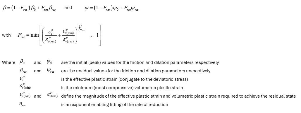
Model 1 - Strain dependent model for SR3/SR4 The strain-dependent variable critical state model for SR3/SR4 models allows to consider a variation in the friction ( β) and dilation ( ψ) parameters according to the following equations:
The input properties are then: • Location 1 - Residual value of beta ( βres) • Location 2 - Residual value of psi ( ψres) • Location 3 - Residual effective plastic strain ( ε(p)res) • Location 4 - Residual volumetric plastic strain ( ε(vp)res) • Location 5 - Exponent ( nres)
Model 2 - Strain dependent model for Anisotropic Rotated SR3 Model • Location 1 - Residual value of beta ( βres) • Location 2 - Residual value of psi ( ψres) • Location 3 - Residual effective plastic strain ( ε(p)res) • Location 4 - Residual volumetric plastic strain ( ε(vp)res) • Location 5 - Exponent ( nres) • Location 6 - Residual value of alpha ( alphares)
|
|||||||||||||||
| Mech_comp_type Type of mechanical compaction model |
Usage |
||||
|
||||
Description |
||||
Mech_comp_type keyword enables to use a mechanical compaction model (such as Athy or Schneider) to automatically and internally generate the corresponding tabular hardening law data that would be required to model the target normal compaction trend under hydrostatic (zero overpressure) conditions. Thus this simplifies the definition of the hardening law for non Cam clay type compaction curves. Valid models are:
• 1 - Schneider compaction trend model • 2 - Athy compaction trend model
|
| Mech_comp_properties Properties defining the compaction model |
Usage |
|||||||||||||||
|
|||||||||||||||
Description |
|||||||||||||||
Properties defining the mechanical compaction models
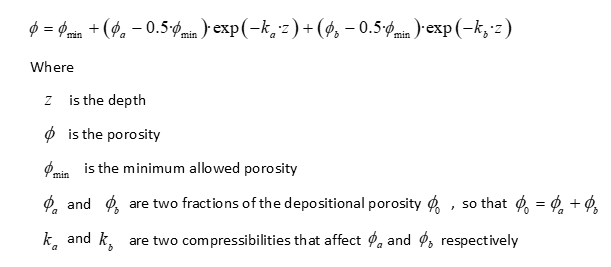
Model 1 – Schneider Model This model defines the evolution of porosity as a function of depth as
The required properties are: • Location 1 - Porosity ( φa) • Location 2 - Porosity ( φb) • Location 3 - Compressibility ( ka) • Location 4 - Compressibility ( kb)
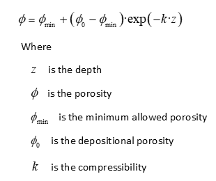
Model 2 – Athy Model This model defines the evolution of porosity as
The required properties are: • Location 1 - Porosity ( φa) • Location 2 - Compressibility ( ka)
|
|||||||||||||||
| Mech_comp_flags Flags for mechanical compaction model |
Usage |
|||||||||||||||
|
|||||||||||||||
Description |
|||||||||||||||
Flags for output of csv files with generated data from mechanical compaction models. Valid values and options are:
The required properties are: • Location 1 - Flag for output .csv files with porosity vs depth (Default 1) • Location 2 - Flag for output .csv files with generated tabular hardening data (Default 1)
|
|||||||||||||||
| Mech_comp_settings Additional settings for the compaction model |
Usage |
|||||||||||||||
|
|||||||||||||||
Description |
|||||||||||||||
Properties used in the internal calculations of the hardening data when using a mechanical compaction model. Input of appropiate values is required to ensure precision in the modelled target normal compaction trend. The appropiate values are material dependent and usually vary with friction angle and flow rule. In order to obtain the aporpiate values a single element k0 test may be initially run with the default values in order to predict the appropiate ones as described in tutorial Mat_001d. The input properties are:
•Location 1 - pc/p' ratio (Default 1.05) •Location 2 - K0 value (Default 0.8)
|
|||||||||||||||
| Mech_comp_max_depth Maximum depth considered for mechanical compaction model |
Usage |
||||
|
||||
Description |
||||
The maximum depth for the compaction model when computing equivalent properties (default 8000m)
|
| Mech_comp_num_points Maximum number of points in mechanical compaction model hardening curve |
Usage |
||||
|
||||
Description |
||||
Defines the maximum number of points for the hardening curve generated for the mechanical compaction model (default 35)
|
| Mech_comp_min_porosity Minimum allowable porosity for mechanical compaction model |
Usage |
||||
|
||||
Description |
||||
Minimum allowable porosity when generating the hardening data associated with the for mechanical compaction model (default 0.01; i.e. 1%)
|
| Viscoplastic_material_type Viscoplasticity type number |
Usage |
||||
|
||||
Description |
||||
Three elasto-viscoplasticity models are available. Valid values are:
• 1 - Herschel-Bulkley type law • 2 - Temperature dependent Herschel-Bulkley type law • 3 - Steady-state salt creep law
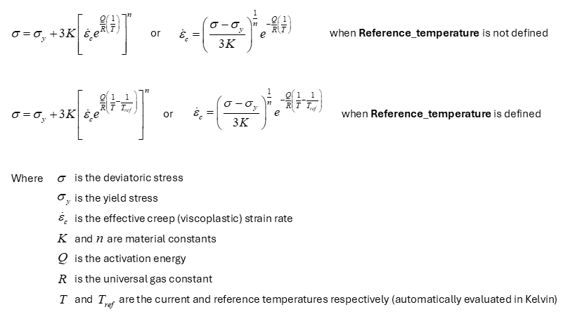
Model 1 - Herschel-Bulkley The Herschel-Bulkley type law is defined as:
Model 2 - Temperature dependent Herschel-Bulkley type law This is the Herschel-Bulkley law (Model 1) augmented by an exponential activation energy term to give a temperature dependent behaviour which is defined by the following equation:
Notes •The reference temperature may be specified using Reference_temperature keyword •Note that a different equation is used depending on whether Reference_temperature is defined or not. Equivalent model behaviour using the two equations may be achieved by scaling the input material contant as:
•Note that the temperatures in the equation are allways evaluated in Kelvin and automatically converted when working with Celcious units •The gas constant should be specified using Gas_constant.
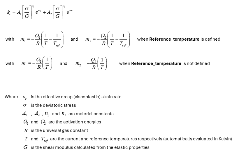
Model 3 - Steady-state salt creep law The steady state salt creep law is defined as:
Notes •The reference temperature may be specified using Reference_temperature keyword •Note that a different equation is used depending on whether Reference_temperature is defined or not. Equivalent model behaviour using the two equations may be achieved by scaling the input material contants as:
•Note that the temperatures in the equation are allways evaluated in Kelvin and automatically converted when working with Celcious temperature units •The gas constant should be specified using Gas_constant. •Shear modulus in Parageo is calculated from Young's modulus and Poisson's ratio. Therefore in order to define a temperature variation in Shear modulus a temperature variation in Young's modulus should be defined via Elastic_properties_tvar (temperature variation Model 1)
|
| Viscoplastic_properties Viscoplastic properties (all models) |
Usage |
|||||||||||||||
|
|||||||||||||||
Description |
|||||||||||||||
The viscoplastic properties are model dependent:
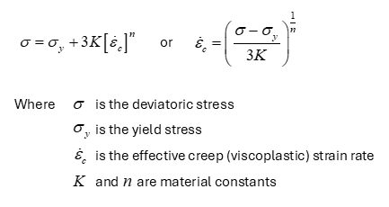
Model 1 - Herschel-Bulkley The Herschel-Bulkley type law is defined as:
Material Properties The viscoplastic properties are: • Location 1 - Yield stress ( σy) • Location 2 - Material constant ( K) • Location 3 - Exponent ( n)
State Variables The default output state variables are: •'V_strn' - Viscoplastic Strain •'V_strn_r' - Viscoplastic Strain Rate •'V_Strs' - Viscoplastic stress •'V_viscos' - Apparent viscosity
Additional state variables that may be requested (see Output_data ) are: •V_flag' - Viscoplastic state •V_strnxx - Viscoplastic Strain XX •V_strnyy - Viscoplastic Strain YY •V_strnzz - Viscoplastic Strain ZZ •V_strnxy - Viscoplastic Strain XY •V_strnyz - Viscoplastic Strain YZ •V_strnzx - Viscoplastic Strain ZX
Model 2 - Temperature dependent Herschel-Bulkley type law This is the Herschel-Bulkley law (Model 1) augmented by an exponential activation energy term to give
Material Properties The viscoplastic properties are: • Location 1 - Yield stress ( σy) • Location 2 - Material constant ( K) • Location 3 - Exponent ( n) • Location 4 - Activation energy ( Q)
State Variables The default output state variables are: •'V_strn' - Viscoplastic Strain •'V_strn_r' - Viscoplastic Strain Rate •'V_Strs' - Viscoplastic stress •'V_viscos' - Apparent viscosity
Additional state variables that may be requested (see Output_data ) are: •V_flag' - Viscoplastic state •V_strnxx - Viscoplastic Strain XX •V_strnyy - Viscoplastic Strain YY •V_strnzz - Viscoplastic Strain ZZ •V_strnxy - Viscoplastic Strain XY •V_strnyz - Viscoplastic Strain YZ •V_strnzx - Viscoplastic Strain ZX
Notes •The reference temperature may be specified using Reference_temperature keyword •Note that a different equation is used depending on whether Reference_temperature is defined or not. Equivalent model behaviour using the two equations may be achieved by scaling the input material contant as:
•Note that the temperatures in the equation are allways evaluated in Kelvin and automatically converted when working with Celcious units •The gas constant should be specified using Gas_constant.
Model 3 - Steady-state salt creep law The steady state salt creep law is defined as:
Material Properties The viscoplastic properties are: • Location 1 - Constant ( A1) • Location 2 - Exponent ( n1) • Location 3 - Activation energy ( Q1) • Location 4 - Constant ( A2) • Location 5 - Exponent ( n2) • Location 6 - Activation energy ( Q2)
State Variables The default output state variables are: •'V_strn' - Viscoplastic Strain •'V_strn_r' - Viscoplastic Strain Rate •'V_Strs' - Viscoplastic stress •'V_viscos' - Apparent viscosity
Additional state variables that may be requested (see Output_data ) are: •V_flag' - Viscoplastic state •V_strnxx - Viscoplastic Strain XX •V_strnyy - Viscoplastic Strain YY •V_strnzz - Viscoplastic Strain ZZ •V_strnxy - Viscoplastic Strain XY •V_strnyz - Viscoplastic Strain YZ •V_strnzx - Viscoplastic Strain ZX
Notes •The reference temperature may be specified using Reference_temperature keyword •Note that a different equation is used depending on whether Reference_temperature is defined or not. Equivalent model behaviour using the two equations may be achieved by scaling the input material contants as:
•Note that the temperatures in the equation are allways evaluated in Kelvin and automatically converted when working with Celcious temperature units •The gas constant should be specified using Gas_constant. •Shear modulus in Parageo is calculated from Young's modulus and Poisson's ratio. Therefore in order to define a temperature variation in Shear modulus a temperature variation in Young's modulus should be defined via Elastic_properties_tvar (temperature variation Model 1)
|
|||||||||||||||
| Regularisation_type Regularization type number |
Usage |
||||
|
||||
Description |
||||
Regularization model type number. Valid values are: • 1 - Fracture Energy model (Default)
|
| Regularisation_properties (or Regularisation_model_1) Regularisation properties for Fracture Energy model |
Usage |
|||||||||||||||
|
|||||||||||||||
Description |
|||||||||||||||
Model 1 - Fracture Energy Regularization Material softening often leads the propagation of localizations, representing shear bands or faults. While the onset of localization may be readily predicted, accurate representation of the propagation of localizations and evaluation of the energy dissipation in the post-localization configuration is, more difficult using standard continuum approaches. This is due to a number of well-documented issues including: •The direction of propagation may be severely biased by the direction of the grid lines; e.g. localizations aligned with the element edges or element diagonals. •Energy dissipation by both mode-I or mode-II deformation on the localization bands is very sensitive to the fineness of the discretization; i.e. the solutions are dependent on the element length scale rather than a physical material length scale. •Large shear movement on the localizations causes excessive mesh distortion which results in termination of the solution unless the domain is remeshed. ParaGeo uses the fracture energy approach, where the global energy dissipation is regularized by including fracture energy ( Gf) as a material constant in the equations governing state variable evolution (Bažant and Oh, 1983). This fracture energy approach arises from linear elastic fracture mechanics (LEFM) and has been adopted by numerous researchers for mode-I fracturing of quasi-brittle materials. Generally, the strain-softening constitutive response includes additional material constants associated with the crack band width and the localization is deemed to occur in the finite volume of the crack band, which ensures finite energy dissipation. Whilst the standard fracture energy approach has been shown to work well for mode-I fracturing of rock and concrete, the characteristic response of some rock types shows significant departure from the assumptions of LEFM. This may be approximately described by assuming that the energy release rate for fracture growth is variable and is defined by a nonlinear resistance curve (Bažant et al., 1993) instead of the constant ( Gf ). Adoption of this concept leads to a simple frictional regularization model (Crook et al., 2003, Pietruszczak and Mróz,1981) of the form:
This expression states that as the element size increases the softening slope becomes steeper. This is consistent with the requirement that the energy dissipated should be approximately independent of the element size; i.e. if larger elements are used, giving larger volumes associated with the failure zone, the strain associated with the deformation must decrease to maintain the same energy dissipation as obtained with a the finer mesh. The fracture energy approach has the advantages that: •Mesh invariance of the global energy dissipation is approximately maintained within an acceptable range of element size. •The approach may be implemented to regularize both mode-I and mode-II localization. •It is straightforward to implement within any finite strain framework and for a range of constitutive models. It must be recognized, however, that although the energy dissipation is mesh size independent the localization limiter is strictly only valid for the Sub-h and Iso-h models; i.e. in models where the localization is equal or less than the characteristic length of the finite elements. Furthermore, in Sub-h simulations the localization is limited to a single band of elements, so that the sharp gradients in the strain field will be poorly approximated if the strain field is evaluated using the standard element interpolation functions. Notwithstanding these limitations, the effectiveness of the regularization methodology in correctly reproducing size effects in mode-II localization has been demonstrated by simulation of thick-walled cylinder (TWC) tests for Berea sandstone and Castlegate sandstone, where the sample internal radii ranged from 8mm to 200mm (Crook et al., 2003).
Material Properties Four regularisation properties are specified: • Location 1 - Characteristic length for material ( lc) • Location 2 - Constant ( A) (Recommended value 0.0) • Location 3 - Exponent ( n) • Location 4 - Maximum allowable change factor ( fallow)
Notes •The value of lcm is dependent on the scale of the simulation. For lab test simulation scale the value of lcm corresponds to the width of a single shear band (e.g. 2 - 3 mm) whereas for field scale simulations the value of lcm should be of the same order of magnitude as the element length.
|
|||||||||||||||
| Diagenesis_reactions List of diagenesis reactions for material |
Usage |
|||||||||||||||
|
|||||||||||||||
Description |
|||||||||||||||
Several diagenetic reactions may be defined and each reaction must be defined using the Diagenesis_data structure. This data is a list of the ID numbers of diagenesis reactions to be used.
|
|||||||||||||||
| Diagenesis_reaction_names List of diagenesis reaction names for material |
Usage |
|||||||||||||||
|
|||||||||||||||
Description |
|||||||||||||||
Several diagenetic reactions may be defined and each reaction must be defined using the Diagenesis_data structure. This data is a list of the diagenesis reactions to be used.
|
|||||||||||||||
| Decompaction_type Decompaction type number |
Usage |
||||
|
||||
Description |
||||
Defines the model for computation of decompaction in a restoration analysis. Valid models are: • 1 - Porosity vs. depth • 2 - Directional decompaction using an imported distribution of strains
|
| Decompaction_spatial ID number of the spatial variation that defines the porosity vs. depth curve for decompaction |
Usage |
||||
|
||||
Description |
||||
Defines the spatial variation (ID number) that defines the porosity vs. depth curve for decompaction.
|
| Decompaction_properties Properties for decompaction |
Usage |
|||||||||||||||
|
|||||||||||||||
Description |
|||||||||||||||
The Decompaction data is dependent on the model type.
Model 1 - Porosity vs. Depth •Location 1 - Maximum increment in porosity in a mechanical step; e.g. 0.0001. This is required to prevent a large jump in porosity in a single step.
Notes •If restoration properties are not defined then the default maximum change is 0.001 •The porosity vs. depth curve should be assigned via Decompaction_spatial
|
|||||||||||||||
| Directional_decomp_type Directional decompaction type number |
Usage |
||||
|
||||
Description |
||||
Defines the model for computation of directional decompaction in a restoration analysis. Valid models are: • 1 - Maximum strain model • 2 - Strain component model
|
| Directional_decomp_properties Properties for directional decompaction |
Usage |
|||||||||||||||
|
|||||||||||||||
Description |
|||||||||||||||
The Decompaction data is dependent on the model type
Model 1 - Maximum strain model The model applies a directional decompaction based on the total volume strain. The direction of the volume strain is appleid in the direction of the most compressive principal strain component •Location 1 - Magnification factor for total volume changes (default 1.0)
Model 2 - Strain component model The model applies a directional decompaction based on the direction volume strain components. •Location 1 - Magnification factor for total volume changes (default 1.0)
|
|||||||||||||||
| Bulk_temp_type Grain temperature dependence type |
Usage |
||||
|
||||
Description |
||||
Grain temperature dependence type, where valid types are: • 1 - Isothermal (Default if temperature variation data is not defined) • 2 - Temperature dependent (Default if temperature variation data is defined)
Notes •If Bulk_temp_type is not specified then by default the grain properties are assumed isothermal
|
| Grain_stiffness Grain stiffness |
Usage |
||||
|
||||
Description |
||||
Defines the grain stiffness in the selected Units
|
| Grain_stiffness_tvar Grain stiffness temperature variation |
Usage |
||||
|
||||
Description |
||||
Grain stiffness temperature variation. A Gradient term defines a linear variation of Grain stiffness ( Grain_stiffness ) with temperature i.e.
|
| Grain_density Grain density |
Usage |
||||
|
||||
Description |
||||
Allows specification of: •Grain density if poroelastic material •Bulk density if non-porous material
|
| Grain_density_tvar Grain density temperature variation |
Usage |
||||
|
||||
Description |
||||
Grain density temperature variation. A Gradient term defines a linear variation of Grain density ( Grain_stiffness ) with temperature i.e.
|
| Singlephase_fluid Single phase fluid assignment |
Usage |
||||
|
||||
Description |
||||
Assigns a single-phase fluid to the pore space of the material. The single-phase fluid properties are defined on the /k1 Fluid_properties data structure.
|
| Singlephase_fluid_name Single phase fluid assignment |
Usage |
||||
|
||||
Description |
||||
Assigns a single-phase fluid to the pore space of the material. The single-phase fluid properties are defined on the Fluid_properties data structure.
|
| Fluid_saturation Initial fluid saturation (default 1.0 - fully saturated) |
Usage |
||||
|
||||
Description |
||||
Initial fluid saturation (default 1.0 - fully saturated)
|
| Biot_type Biot constant type number |
Usage |
||||
|
||||
Description |
||||
Defines the method (by number) to be used to define the Biot constant. The valid methods are: • 1 - constant specified Biot Constant (Default) • 2 - porosity dependent Biot Constant
|
| Biot_properties Data defining the Biot constant |
Usage |
|||||||||||||||
|
|||||||||||||||
Description |
|||||||||||||||
Data defining the Biot constant. Generally: •Location 1 - Biot constant
|
|||||||||||||||
| Biot_vs_porosity Biot constant vs. porosity table |
Usage |
|||||||||||||||
|
|||||||||||||||
Description |
|||||||||||||||
Biot constant vs. porosity table. The data is provided as a 2-D table where: •Location 1 - List of porosities •Location 2 - Biot constant for each porosity specified in Row 1
|
|||||||||||||||
| Permeability_type Permeability type number (1-constant, 2-perm vs. porosity, 3-perm vs. pore pressure) |
Usage |
||||
|
||||
Description |
||||
Permeability model type number. Valid models comprise: • 1 - constant permeability (Default) • 2 - User defined permeability vs. porosity curve in a tabular form • 3 - permeability vs. pore pressure curve (Generally only for single-field porous flow analysis where geomechanical deformation is not computed) • 4 - permeability vs. effective mean stress (coupled analysis only) • 5 - Power Law analytical model • 6 - Kozeny-Carman analytical model • 7 - Exponential analytical model • 8 - Yang and Aplin permeability function for clay fraction
|
| Permeability_properties Permeability properties |
Usage |
|||||||||||||||
|
|||||||||||||||
Description |
|||||||||||||||
The Permeability properties are dependent on the model type:
Model 5 - Power Law The power law model defines permeability as:
The Permeability properties for power law comprise (2 values required): • Location 1 - "Pre-multiplier" • Location 2 - "Exponent"
Below it is shown that with a value of n =4.5 the slope of the Power Law permeability model allows to aproximate kozeny-Carman curves by choosing appropiate "A" values (Kozeny-Carmen curves in the plot are for average sand, siltstone and shale according to Hantschel and Kauerauf (2009); grey discontinous curves show Yang and Apling curves for clay fractions of 0.0, 0.2, 0.4, 0.6, 0.8 and 1.0).
State Variables The input and output state variables are: •"Prmltplr" - Pre-multiplier •"Exponent" - Exponent
Model 6 - Kozeny-Carman The Kozeny-Carman model defines permeability as a function of porosity as:
The Permeability properties for Kozeny-Carman comprise (3 values required): • Location 1 - "Pre-multiplier" • Location 2 - "Exponent 1" • Location 2 - "Exponent 2"
The classical Kozeny-Carman curves take values of n =3 and m =2. The permeability pre-multiplier it is often computed as:
State Variables The input and output state variables are: •"Prmltplr" - Pre-multiplier •"Exponen1" - Exponent 1 (n) •"Exponen2" - Exponent 2 (m)
It should be noted that the K-C curves for Sandstone, Siltstone and Shale according to Hantschel and Kauerauf (2009) which are plotted for reference in several figures here use a modified expression of the Kozeny-Carman model proposed by Ungerer et al. (1990). Below it is shown a comparison of the model implemented in ParaGeo compared with those curves.
Model 7 - Exponential The exponential permeability model (e.g. Nygard et al. (2004)) defines permeability as a function of porosity as:
The Permeability properties for the exponential law comprise (2 values required): • Location 1 - "Permeability project to zero porosity" • Location 2 - "Material constant"
Nygard et al. (2004) derived empirical parameters from experiments on several clays (grey discontinous curves show Yang and Apling curves for clay fractions of 0.0, 0.2, 0.4, 0.6, 0.8 and 1.0 which are plotted for reference):
State Variables The input and output state variables are: •"Permzpor" - Permeability project to zero porosity •"Matconst" - Material constant
Model 8 - Yang and Aplin The Yang and Aplin (2010) model defines permeability as a function of void ratio and clay fraction as:
The Permeability properties for Yang and Aplin comprise: • Location 1 - "Clay fraction (range 0.0 < CF < 1.0)"
See below the plot of Yang and Apling curves for different values of clay fraction (CF):
State Variables The input and output state variables are: •"Clayfrac" - Clay fraction
|
|||||||||||||||
| Orthotropic_permeability_type Orthotropic permeability type |
Usage |
||||
|
||||
Description |
||||
Defines whether the permeability model is isotropic or orthotropic. Valid models comprise: • 1 - isotropic (Default if no orthotropic data is defined) • 2 - orthotropic (Default)
|
| Perm_interpolation_type Permeability interpolation type |
Usage |
||||
|
||||
Description |
||||
Defines whether the permeability model is linearly interpolated or logaritmically iterpolated. Valid models comprise: • 0 - Lienar interpolation (Default if no data is defined) • 1 - Log linear interpolation
|
| Permeability Isotropic constant permeability |
Usage |
||||
|
||||
Description |
||||
Isotropic constant permeability value
|
| Permeability_x Constant permeability in X direction |
Usage |
||||
|
||||
Description |
||||
Constant permeability in X direction for orthotropic materials
|
| Permeability_y Constant permeability in Y direction |
Usage |
||||
|
||||
Description |
||||
Constant permeability in Y direction for orthotropic materials
|
| Permeability_z Constant permeability in Z direction |
Usage |
||||
|
||||
Description |
||||
Constant permeability in Z direction for orthotropic materials
|
| Permeability_vs_porosity Isotropic permeability vs porosity curve |
Usage |
|||||||||||||||
|
|||||||||||||||
Description |
|||||||||||||||
Isotropic Porosity dependent permeability. The data is provided as a 2-D table where: •Row 1 - list of porosities •Row 2 - permeability for each porosity specified in Row 1
|
|||||||||||||||
| Permeability_x_vs_porosity X direction permeability vs porosity curve |
Usage |
|||||||||||||||
|
|||||||||||||||
Description |
|||||||||||||||
X direction Porosity dependent permeability. The data is provided as a 2-D table where: •Row 1 - list of porosities •Row 2 - permeability for each porosity specified in Row 1
|
|||||||||||||||
| Permeability_y_vs_porosity Y direction permeability vs porosity curve |
Usage |
|||||||||||||||
|
|||||||||||||||
Description |
|||||||||||||||
Y direction Porosity dependent permeability. The data is provided as a 2-D table where: •Row 1 - list of porosities •Row 2 - permeability for each porosity specified in Row 1
|
|||||||||||||||
| Permeability_z_vs_porosity Z direction permeability vs porosity curve |
Usage |
|||||||||||||||
|
|||||||||||||||
Description |
|||||||||||||||
Z direction Porosity dependent permeability. The data is provided as a 2-D table where: •Row 1 - list of porosities •Row 2 - permeability for each porosity specified in Row 1
|
|||||||||||||||
| Perm_anisotropy_factor Factor of horizontal to vertical permeability |
Usage |
||||
|
||||
Description |
||||
Defines the factor ( forth) of horizontal to vertical permeability. Currently only used for analytical and user defined models.
|
| Min_permeability_cutoff Minimum permeability cutoff |
Usage |
||||
|
||||
Description |
||||
Min_permeability_cutoff allows to constrain the minimum allowed permeability value when using analytical permeability models. Ongoing compaction after the Min_permeability_cutoff value has been achived will not cause further reduction in permeability. By default the minimum permeability value is unconstrained.
|
| Max_permeability_cutoff Maximum permeability cutoff |
Usage |
||||
|
||||
Description |
||||
Max_permeability_cutoff allows to constrain the maximum allowed permeability value when using analytical permeability models. Porosity increase (dilation) after the Max_permeability_cutoff value has been achived will not cause further increase in permeability. By default the maximum permeability value is unconstrained.
|
| Permeability_vs_saturation_type Saturation type number |
Usage |
||||
|
||||
Description |
||||
Permeability vs. saturation model type. Only one model is available: • 1 - Permeability multiplication factor vs. saturation curve.
|
| permeability_vs_saturation Permeability vs. saturation curve |
Usage |
|||||||||||||||
|
|||||||||||||||
Description |
|||||||||||||||
Defines a multiplication factor for permeability ( 0.0 ≤ fmult ≤ 1.0) vs. pore space saturation. The data is provided as a 2-D table where: •Row 1 - list of fluid saturations •Row 2 - permeability multiplication factor for each saturation specified in Row 1
|
|||||||||||||||
| Saturation_type Saturation vs. pore pressure model type |
Usage |
||||
|
||||
Description |
||||
Model type for defining the relationship between saturation and pore pressure. Only one model is available: • 1 - Saturation vs. pore pressure curve
|
| Saturation_vs_pore_pressure Saturation vs. pore pressure curve |
Usage |
|||||||||||||||
|
|||||||||||||||
Description |
|||||||||||||||
Saturation vs. pore pressure curve. The data is provided as a 2-D table where: •Row 1 - list of pore fluid pressures •Row 2 - saturation for each pore pressure specified in Row 1
|
|||||||||||||||
| Permeability_vs_pressure Isotropic permeability vs. Pore Pressure |
Usage |
|||||||||||||||
|
|||||||||||||||
Description |
|||||||||||||||
Isotropic permeability vs. pore pressure curve. The data is provided as a 2-D table where: •Row 1 - list of pore pressures •Row 2 - permeability for each pore pressure specified in Row 1
|
|||||||||||||||
| Permeability_x_vs_pressure X direction permeability vs. Pore Pressure |
Usage |
|||||||||||||||
|
|||||||||||||||
Description |
|||||||||||||||
X direction permeability vs. pore pressure curve. The data is provided as a 2-D table where: •Row 1 - list of pore pressures •Row 2 - permeability for each pore pressure specified in Row 1
|
|||||||||||||||
| Permeability_y_vs_pressure Y direction permeability vs. Pore Pressure |
Usage |
|||||||||||||||
|
|||||||||||||||
Description |
|||||||||||||||
Y direction permeability vs. pore pressure curve. The data is provided as a 2-D table where: •Row 1 - list of pore pressures •Row 2 - permeability for each pore pressure specified in Row 1
|
|||||||||||||||
| Permeability_z_vs_pressure Z direction permeability vs. Pore Pressure |
Usage |
|||||||||||||||
|
|||||||||||||||
Description |
|||||||||||||||
Z direction permeability vs. pore pressure curve. The data is provided as a 2-D table where: •Row 1 - list of pore pressures •Row 2 - permeability for each pore pressure specified in Row 1
|
|||||||||||||||
| Permeability_user User permeability data |
Usage |
|||||||||||||||
|
|||||||||||||||
Description |
|||||||||||||||
User permeability data defined as a two-dimensional table of values. The user permeability data can only be used in conjunction with the ParaGeo User defined Plug-In functionality.
|
|||||||||||||||
| Grain_conductivity_type Conductivity type number (1-isotropic, 2-orthotropic) |
Usage |
||||
|
||||
Description |
||||
Thermal conductivity model type. Two models are available: • 1 - Isotropic (Default if no orthotropic data defined) • 2 - Orthotropic (Default if orthotropic data defined)
|
| Grain_cond_temp_type Conductivity temperature dependence type |
Usage |
||||
|
||||
Description |
||||
Thermal conductivity temperature dependent model type. Valid types are: • 1 - Isothermal (Default if temperature variation data not defined) • 2 - Temperature dependent (Default if temperature variation data defined)
|
| Grain_conductivity Isotropic grain conductivity |
Usage |
||||
|
||||
Description |
||||
Isotropic grain conductivity
|
| Grain_conductivity_x Isotropic or X direction grain conductivity |
Usage |
||||
|
||||
Description |
||||
X direction grain conductivity
|
| Grain_conductivity_tvar Isotropic grain conductivity variation |
Usage |
||||
|
||||
Description |
||||
Isotropic grain conductivity variation. A Gradient term defines a linear variation of Grain conductivity ( Grain_conductivity ) with temperature i.e.
|
| Grain_conductivity_x_tvar Grain conductivity variation with temperature in x direction |
Usage |
||||
|
||||
Description |
||||
Grain conductivity variation in the x direction. A Gradient term defines a linear variation of Grain conductivity ( Grain_conductivity or Grain_conductivity_x) with temperature i.e.
|
| Grain_conductivity_y Grain conductivity in Y direction |
Usage |
||||
|
||||
Description |
||||
Grain conductivity in Y direction
|
| Grain_conductivity_y_tvar Grain conductivity variation with temperature in y direction |
Usage |
||||
|
||||
Description |
||||
Y direction grain conductivity variation. A Gradient term defines a linear variation of Grain conductivity ( Grain_conductivity or Grain_conductivity_y) with temperature i.e.
|
| Grain_conductivity_z Grain conductivity in Z direction |
Usage |
||||
|
||||
Description |
||||
Grain conductivity in Z direction
|
| Grain_conductivity_z_tvar Grain conductivity variation with temperature in Z direction |
Usage |
||||
|
||||
Description |
||||
Z direction grain conductivity variation. A Gradient term defines a linear variation of Grain conductivity ( Grain_conductivity or Grain_conductivity_z) with temperature i.e.
|
| Grain_specific_heat Grain specific heat |
Usage |
||||
|
||||
Description |
||||
Grain specific heat
|
| Grain_specific_heat_tvar Grain specific heat temperature variation |
Usage |
||||
|
||||
Description |
||||
Grain specific heat temperature variation. A Gradient term defines a linear variation of Grain specific heat ( Grain_specific_heat) with temperature i.e.
|
| Linear_therm_exp_type Linear thermal expansion model type |
Usage |
||||
|
||||
Description |
||||
Linear thermal expansion model type. Valid types are: • 1 - Isotropic (Default if no orthotropic data defined) • 2 - Orthotropic (Default if orthotropic data defined) • 3 - Isotropic (defining coefficients as state variables) • 4 - Orthotropic (defining coefficients as state variables)
Notes •Models 3 and 4 are identical to models 1 and 2 respectively, but allow assignment of spatially varing expansion coefficients
|
| Linear_therm_exp_temp_type Linear thermal expansion temperature dependence type |
Usage |
||||
|
||||
Description |
||||
Linear thermal expansion temperature dependence type. Valid types are: • 1 - Isothermal (Default if temperature variation data not defined) • 2 - Temperature dependent (Default if temperature variation data defined)
|
| Linear_therm_exp_coeff Isotropic linear thermal expansion coefficient |
Usage |
||||
|
||||
Description |
||||
Isotropic linear thermal expansion coefficient
|
| Linear_therm_exp_coeff_x Isotropic grain or X direction linear thermal expansion coefficient |
Usage |
||||
|
||||
Description |
||||
Linear thermal expansion coefficient in x direction
|
| Linear_therm_exp_coeff_tvar Isotropic Linear thermal expansion coefficient variation with temperature |
Usage |
||||
|
||||
Description |
||||
Isotropic Linear thermal expansion coefficient variation with temperature. A Gradient term defines a linear variation of Grain thermal expansion coefficient ( Linear_therm_exp_coeff ) with temperature i.e.
|
| Linear_therm_exp_coeff_x_tvar X direction Linear thermal expansion coefficient variation with temperature |
Usage |
||||
|
||||
Description |
||||
Linear thermal expansion coefficient variation with temperature in x direction. A Gradient term defines a linear variation of Grain thermal expansion coefficient ( Linear_therm_exp_coeff_x) with temperature i.e.
|
| Linear_therm_exp_coeff_y Y direction Linear thermal expansion coefficient |
Usage |
||||
|
||||
Description |
||||
Linear thermal expansion coefficient in y direction
|
| Linear_therm_exp_coeff_y_tvar Y direction Linear thermal expansion coefficient variation with temperature |
Usage |
||||
|
||||
Description |
||||
Linear thermal expansion coefficient variation with temperature in y direction. A Gradient term defines a linear variation of Grain thermal expansion coefficient ( Linear_therm_exp_coeff_y) with temperature i.e.
|
| Linear_therm_exp_coeff_z Z direction Linear thermal expansion coefficient |
Usage |
||||
|
||||
Description |
||||
Linear thermal expansion coefficient in z direction
|
| Linear_therm_exp_coeff_z_tvar Z direction Linear thermal expansion coefficient variation with temperature |
Usage |
||||
|
||||
Description |
||||
Linear thermal expansion coefficient variation with temperature in z direction. A Gradient term defines a linear variation of Grain thermal expansion coefficient ( Linear_therm_exp_coeff_z) with temperature i.e.
|
| Grain_therm_exp_type Grain thermal expansion temperature dependence type |
Usage |
||||
|
||||
Description |
||||
Grain thermal expansion temperature dependence type. Valid types are: • 1 - Isothermal (Default if temperature variation data not defined) • 2 - Temperature dependent (Default if temperature variation data defined)
|
| Grain_therm_exp_coeff Isotropic grain thermal expansion coefficient |
Usage |
||||
|
||||
Description |
||||
Isotropic grain thermal expansion coefficient. The grain thermal expansion coefficient is used in conjunction with the bulk and fluid thermal expansion coefficients to evaluate the rate of pore pressure change in the porous flow field.
|
| Grain_therm_exp_coeff_tvar Isotropic grain thermal expansion coefficient variation with temperature |
Usage |
||||
|
||||
Description |
||||
Grain Bulk thermal expansion coefficient variation with temperature. A Gradient term defines a linear variation of Grain thermal expansion coefficient ( Grain_therm_exp_coeff ) with temperature i.e.
|
| Fracture_sets List of fracture sets |
Usage |
|||||||||||||||
|
|||||||||||||||
Description |
|||||||||||||||
List of fracture sets assigned to material by number
|
|||||||||||||||
| Fracture_set_names List of fracture sets |
Usage |
|||||||||||||||
|
|||||||||||||||
Description |
|||||||||||||||
List of fracture sets assigned to material by names
|
|||||||||||||||

