The objective in this case is to achieve a quasi-static solution.  This necessitates:

1Increasing the natural frequency of the system; i.e. allowing the stress applied  at the top of the model to propagate more quickly through the model.   Increasing the natural frequency lowers the critical time step and therefore increases the number of time steps within the time range 0.0 < t < 2.0.

2Ensuring that the frequency of loading is as low as possible; i.e. applying smooth load functions, to minimize dynamic deformation induced by changes in load.

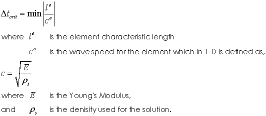
The critical time step is dependent on both the material properties and the size of the elements and for 1-D wave propagation is defined as

 

By Default fmass = 1.0 so that ρs = ρ. Based on this value the critical time step in Case 1A  is Δtcrit = 0.83 so that Δt = fcritΔtcrit = 0.58 and only four steps are required to reach the termination time t=2.0.  In quasi-static problems, mass-scaling can be used to increase the natural frequency, and therefore reduce the critical time step, via:

 

1Specifying fmass < 1.0 via the Initial_mass_scaling_constant in the Material_data data structure.  This reduces the solution mass of all elements in the group but results in a variable element critical time step (as the critical time step is also dependent on the characteristic length of each element)

 

2Specifying a target time step (Δttarg) using the Time_scaling_factors data structure (Abaqus *TIME SCALING keyword).  This increases the solution mass for any element where fcritΔtcrit < Δttarg so that fcritΔtcrit = Δttarg

 

The initial mass-scaling constant scales the mass used to compute the dynamic solution, but does not affect loading (i.e. gravity loads).   The scaling magnitude must be sufficient to reduce the time step close to, or below, the desired value Δttarg. This can be verified by plotting the element critical time step values in ParaView. The time scaling factor is then used to increase the mass of any element so that fcritΔtcrit = Δttarg where Δttarg is the target time step.  Note that elements where fcritΔtcrit > Δttarg are not scaled.

 

The objective is to set the target time step and load ramp data such that the dynamic response is minimized and an approximately quasi-static response is predicted.   In this first case the target time step is set to give approximately 100 steps for ramp time (1.0) defined for load case 1.

 

A more straightforward approach is available in ParaGeo by which an "optimal" time step is defined. This "optimal" algorithm automatically computes the required mass-scaling and time scaling for all elements in the domain so that fcritΔtcrit = Δttarg. This method is easier to set and is generally recommended.

 

 

TIME SCALING

The *TIME SCALING keyword is added to the data file.

 

The equivalent ParaGeo data structure generated is Time_scaling_factors.

 

 

The results are visualized by plotting the high definition history data for global energy and points output in files mech_001_2d_Case1b_000.hdh and mech_001_2d_Case1b_001.hdh respectively.   This data can be pasted into excel workbook mech_001.xls.   Note that as the history files are comma delimited the Excel data import must be modified via Data->Text to Columns->Delimited->Comma.

 

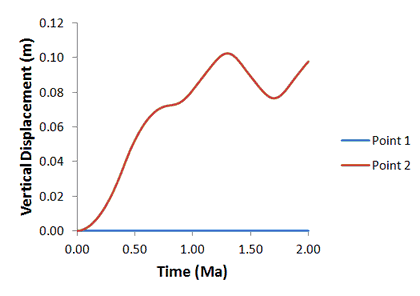
As the surface load is a linear ramp between t=0.0 and t=1.0, the target quasi-static solution is a linearly increasing displacement between t=0.0 and t=1.0 followed by constant displacement. The displacement for point 2, corresponding to the top of the column, however, exhibits a strongly dynamic response between time 1.0 and 2.0.

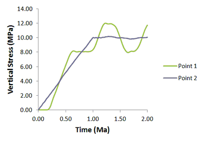
The dynamic response is also evident from the evolution of stress.   The vertical stress at the base of the column remains almost zero until ca. t=0.2 and then subsequently overshoots the vertical stress at point 1 at ca. t=0.6.  The delay is due to the time taken for the stress wave to arrive at the base of the column.  The oscillatory response between time 1.0 and 2.0 is also evident.

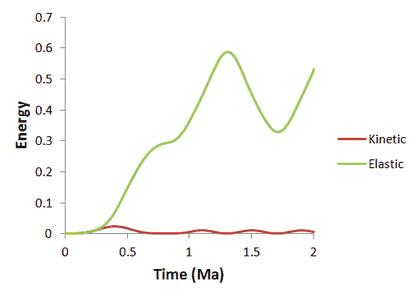
Similarly, the global energy exhibits a low frequency oscillatory response between time 1.0 and 2.0.