Case04 Spatial basal heat flow

Contents

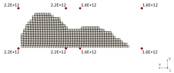
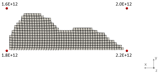
In the present case a spatially varying heat flux will be prescribed to the base of the model during the forward simulation using a Spatial_grid applied via a Spatial_boundary. Two different grids defined within the corresponding .spat files will be used to assign different values at different stages of the simulation:

•Geol_002b_Case04a_BasalHeatFlow_01.spat defining the prescribed basal heat flux distribution for stages 1 to 6

•Geol_002b_Case04a_BasalHeatFlow_02.spat defining the prescribed basal heat flux distribution for stages 7 to 10

Note that only the data relevant to the application of the basal heat flux will be described here.

Spatial grids

Geol_002b_Case04a_BasalHeatFlow_01.spat

The spatial grid defining basal heat fluxes for stages 1 to 6 is shown below.

Data File

* Spatial_grid NUM=101

! ----------------------------------------

Name "Basal_Flux"

Type "Plan1"

Num_division_x 3

Num_division_y 1

Plan_variables IDM=1

"Tm_flux"

Plan_points IDM=2 JDM=8

28000 65000

54000 65000

60000 65000

80000 65000

28000 82000

54000 82000

60000 82000

80000 82000

Plan_values IDM=1 JDM=8

1.6E+12

2.2E+12

1.6E+12

2.2E+12

• The Type for a spatial grid defining basal fluxes must be set as Plan1 (compulsory). This defines the variable values at specified X and Y points (in plan view).

•In the present case the grid contains 3 divisions along the X direction and 1 in the Y direction. Consequently the number of points to be defined will be (3+1) * (1+1) = 8 points.

•The variable being defined via the grid is "Tm_flux" which corresponds to thermal flux.

•The present grid defines a constant value of 1.6E+12 J · m-2 · Ma-1 for 28000 m ≤ X ≤ 54000 m, a constant value of 2.2E+12 J · m-2 · Ma-1 for 60000 m ≤ X ≤ 80000 m and then there will be a gradual change from those values for 54000 m ≤ X ≤ 60000 m

Geol_002b_Case04a_Fig03

View of the initial geometry (from the base) with the defined grid points values

Geol_002b_Case04a_BasalHeatFlow_02.spat

The spatial grid defining basal heat fluxes for stages 7 to 10 is shown below.

Data File

* Spatial_grid NUM=101

! ----------------------------------------

Name "Basal_Flux"

Type "Plan1"

Num_division_x 1

Num_division_y 1

Plan_variables IDM=1

"Tm_flux"

Plan_points IDM=2 JDM=4

32000 65000

80000 65000

32000 82000

80000 82000

Plan_values IDM=1 JDM=4

2.2E+12

1.8E+12

2.0E+12

1.6E+12

•The present grid contains a single cell defined by 4 points.

•The values are defined to decrease from 2.2E+12 J · m-2 · Ma-1 to 1.8E+12 J · m-2 · Ma-1 along the X direction (from 28000 m ≤ X ≤ 80000 m) and decrease by 0.2E+12 J · m-2 · Ma-1 to along the Y direction at the same coordinates. Consequently a WSW - ENE gradient will be imposed.

Geol_002b_Case04a_Fig04

View of the initial geometry (from the base) with the defined grid points values

Spatial boundary

Note that the spatial grids are read using the data structure * Include. The values from the grid are prescribed to the base of the model using a Spatial_boundary data structure.

Data File

* Spatial_boundary NUM=3

! ---------------------------

Name "Basal_heat_flow"

File_name "Geol_002b_Case04a_BasalHeatFlow_01.spat"

Boundary_type "Spatial_grid"

Time_curve "Step_constant"

Conforming_mesh_flag 0

Spatial_grids IDM=1

"Basal_Flux"

Geometry_sets IDM=1

"Basal_surface"

Prescribed_components IDM=1 JDM=1

•The time curve is defined as "Step_constant" (constant full values applied during the whole stage)

•Conforming_mesh_flag set to 0 indicates that the values are defined on an arbitrary grid that does not correspond to the mesh of the model.

•The spatial grid named "Basal_Flux" is defined as the grid that contains the values to be prescribed

•The base of the model is identified by specifying the corresponding geometry set.

•The prescribed component is set as 9 (thermal flux normal to the base).

Results

The results for the forward simulation are provided in Geol_002b\Case04\Results. Note that only a selection of results are provided. The plot files at different times may be visualised by loading the file Geol_002b_Case04a_fsim.xmf in ParaView.

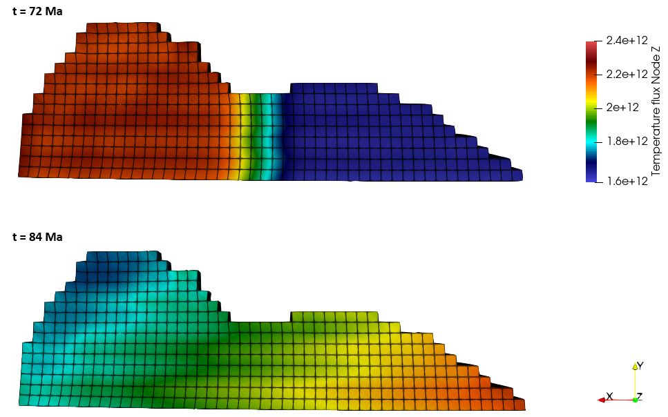
The picture below shows the nodal temperature flux in Z direction viewed at the base of the model. It can be seen as the distribution and the values at the two displayed times are consistent with the two grids defined to prescribe the basal heat flow. It should be noted that the basal heat flow is prescribed normal to the element facet direction. Consequently the values may vary slightly with the ones being prescribed if the facets are not flat. Note also that the range of values exceeds the maximum prescribed value (e.g. see the figure for t=72 Ma). This is because the contrast of thermal conductivities in different layers, the anisotropic properties of the materials (larger thermal conductivity in horizontal direction) and the different thickness in the different layers contribute to a non-vertical heat flux pathways.

Geol_002b_Case04a_Fig01

View of the base of the model at two different times which consider two different basal heat flux distributions

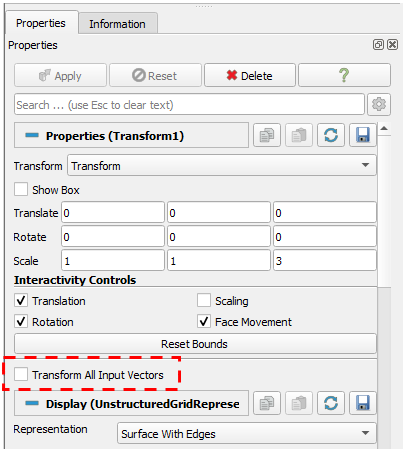
Note that the temperature flux variable is output as a vector and X, Y , Z and Magnitude components may be plotted in ParaView. When plotting vector variables, if a Transform filter with scaling is used (e.g. to show the results with a given vertical exaggeration) care must be taken to deactivate the "Transform All Input Vectors" tick-box option, otherwise the magnitudes of the vector variables will also be accordingly scaled.

Geol_002b_Case04a_Fig02

View of the Transform filter options