Case01 Definition of the SR4 Hardening Table
In some geological-time scale modelling scenarios it may be required to characterise a material with a normal compaction trend that may not be easily modelled by means of the Cam-Clay type analytical hardening discussed in Mat_001b tutorial example. For example, in the following figure an Athy compaction curve for a typical shale is displayed (with depositional porosity Ø0 = 0.7 and compressibility k = 0.83 Km-1) and the analytical hardening model is used to attempt to fit the curve. With the analytical curve number 1 (red curve) a reasonable good fit is obtained for depths shallower than ~1.5 km but porosities are underestimated at greater depths. In order to model less compaction, the hardening parameter lambda (λ) may be decreased but then the modelled porosity drifts from the target at shallower depths (see for example the green curve). One may decrease the depositional porosity and adjust the hardening parameter lambda (λ) in order to obtain a good fit of the modelled porosities with the data for a given target depth interval but both, shallower and deeper porosities than the target interval will show differences with the data (e.g. see the blue curve optimized for a depth interval from c.a. 2 to 3.5 km). It should be noted that the analytical hardening model (Cam-Clay type model) was originally developed to capture the experimental geomechanical behaviour of clays in the lab, ignoring geological-time scale processes that may contribute to the compaction of sediments in nature and are inherently/implicitly included into the compaction curves often assumed in basin modelling.
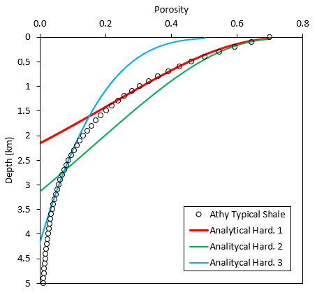
Comparison of an Athy curve for a typical shale and 3 different curves using the analytical hardening model. Note all the curves assumed the same parameters with the only variation being the hardening parameter Lambda (λ) and depositional porosity. A grain density of 2700 Kg/m3 and a water density of 1000 Kg/m3 is assumed.
In those cases we can use the user-defined hardening model in which the user inputs the values of pre-consolidation pressure (pc) and tensile intercept (pt) as a function of the volumetric plastic strain (εvp). However this is not straightforward as:
1.During compaction both, elastic and plastic volumetric strain contribute to the porosity loss
2.To estimate the value of pc for a given porosity it is required to know the effective mean stress (p'), hence to know the vertical and horizontal effective stresses, and the constitutive relationship between p' and pc in a k0 burial path which will depend on the shape of the yield and flow potential surfaces
This tutorial case aims to illustrate how to calculate the hardening input table parameters from any target compaction curve (porosity-depth curve) using an excel sheet. First the details of the calculations performed in the spreadsheet are described and then a step by step guide on how to use the spreadsheet to define and validate the material with an example is provided. Then, an exercise is proposed to the user.
| Calculations in the Excel Sheet |
Here the calculations performed in the excel sheet Mat_001c_Case01a.xlxs are explained in detail. Note that the calculations are performed in depth increments from depositional depth (z = 0 m) to the current evaluated depth point. Note that as the procedure involves calculating non-linear equations the depth increments in the spreadsheet need to be small enough to avoid excessive error due to linear approximation (e.g. 10 m for a 10 Km scale curve, so that we have 1000 points).
The procedure in the spreadsheet is summarized as follows:
1.Define the target compaction curve that we want to model as our Normal Compaction Trend (NCT). This provides the porosity value at each depth. In the current excel sheet an Athy curve is used but any depth porosity curve may be defined.
2.Define the reference pre-consolidation pressure (pc0). This is the pre-consolidation pressure value that corresponds to the reference/depositional porosity.
3.Define grain and fluid densities ( ρg and ρw respectively).
4.Calculate the hydrostatic and lithostatic pressures at each depth (known porosity and grain and fluid density values we can integrate densities) and hence calculate the vertical effective stress (σy') at each depth point.
5.Input an initial guess of k0 ratio (ratio of horizontal to vertical effective stress in uniaxial burial conditions). Recommended initial guess value from 0.7 to 0.8. Note that the true value will depend of the yield and flow potential surfaces shape.
6.Calculate the effective mean stress (p') at each depth according to:
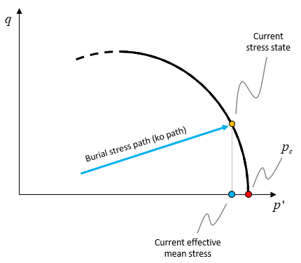
7.Input an initial guess of the ratio between pre-consolidation pressure and effective mean stress (pc/p') in uniaxial burial conditions (k0 path). See the figure below for a graphical representation. The recommended initial guess value of 1.05. Note that the true value will depend on the yield and flow potential surfaces shape.
Schematic of the relationship between the pre-consolidation pressure and the current effective mean stress during burial conditions
8.Calculate the pre-consolidation pressure at each depth as:
9.Calculate the total volumetric strain between the current porosity (Ø) and the initial/depositional porosity (Ø0) as:
10.Input the poro-elastic law parameters reference bulk modulus (K0), kappa (κ) and Aun factor as well as Poisson's ratio (ν). Note that Poisson's ratio is not actually required for calculating the hardening law, but is used in the spreadsheet to derive Young's modulus from Bulk modulus.
11.Calculate the bulk modulus at each depth according to the poro-elasticity law as:
12.Calculate the increment in elastic volumetric strain between two consecutive depth points as:
13.Calculate the accumulated elastic volumetric strain by summing the elastic volumetric strain increments from previous depths to current depth
14.Calculate the plastic volumetric strain for the current depth/porosity as:
In steps 8 and 14 we have calculated pc and εvp which are required parameters for definition of the hardening law. Currently in ParaGeo it is assumed that the tensile intercept cannot increase by means of mechanical compaction so that a constant value is defined in the spreadsheet. Note also that the input value for the top surface stress to be defined in Stratigraphy_surface_load is used as the initial value for the lithostatic stress to ensure consistency with the simulations.
Notes
•The calculations are performed on small depth increments too avoid excessive approximation error in non-linear incremental calculations. Then the values to be input in the ParaGeo material data file are extracted using a lookup table. •The input top surface stress to be defined in Stratigraphy_surface_load is used as the initial value for the lithostatic stress to ensure consistency with the simulations. •The calculations provide the hardening curve for compaction (pority decreasing from the reference/depositional porosity). The hardening curve portion corresponding to dilation due to softening to residual strength values (porosities higher than the reference values) is manually defined. In the spreadsheet increasing slope between consecutive points is considered in order to ensure a smooth curve to avoid numerical instabilities. •The procedure involved input of two initial guess values for constitutive parameters effective stress ratio k0 and ratio of the pre-consolidation pressure to the effective mean stress in a k0 stress path (pc/p'). Those values will provide an initial hardening table that can be input in an initial material definition. Then a small single element oedometer test may be simulated to plot the real predicted values and update them in the spreadsheet to obtain a more accurate hardening table. Then it is recommended to validate the material characterisation by simulating a drained consolidation test and compare the predicted porosity trend with the target one.
|
| Step by Step on how to use the spreadsheet Mat_001c_Case01a |
In this section we demonstrate how to use the excel sheet Mat_001c_Case01a.xlxs in order to define the hardening law corresponding to a target compaction trend. To that end we will use the Athy's typical shale trend that we could not model via the analytical hardening as our target (see the first figure in this example). This compaction curve is obtained using Athy's equation formulated with hydrostatic depth:
Ø = Ø0 · exp(-k· z)
Where Ø is the porosity at the hydrostatic depth z, Ø0 is the depositional porosity and k is the compressibility (Ø0=0.7 and k=0.83 km-1 for the present example; values obtained from Hantschel and Kauerauf, 2009).
The step by step procedure is then as follows:
1.In cells C9 and C10 define the input parameters to calculate the Athy compaction curve.
2.In blue cells from C13 to C23 define the requested input parameters (do not change cell C14) that must be consistent with the values defined in the Material_data with the following recommendations: a.The minimum value for reference pc of should be 0.2 MPa with a recommended value of 0.5 MPa (cell C13) b.The reference bulk modulus set to 100 MPa (cell C17) c.Aun parameter is recommended to be set to 0 for geological applications (cell C19). This will make the bulk modulus solely dependent on pc and not on p' which will prevent excessive stiffness decrease during erosion and uplift due to unloading. d.The initial recommended guess values for k0 and pc/p' are 0.8 and 1.05 respectively (cells C21 and C22 respectively). e.The top surface load boundary condition (to be defined within Stratigraphy_surface_load data structure in ParaGeo data file) is recommended to be set as the pre-consolidation pressure value. This value is to prevent top surface instability in coupled simulations due to the development of tensional stresses in the top surface. This value may be increased if required. Note that to ensure accuracy in the definition of the hardening law the value input in the excel sheet should be the same as the value defined in the data file.
3.Copy cells from I25 to AQ27 and paste it to the material data file within the user-defined hardening law data (see the example below).
View of the first 4 columns of data for user defined hardening in the excel sheet and in the material data file
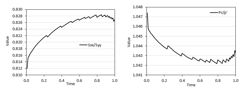
4.Run the Mat_001c_Case01a_k0_test.dat simulation. This is a single element oedometer test. Paste the history point results from the simulation in the sheet "ko test", cell AA33 (including headers). From the plots we can derive more accurate values for k0 (Sxx/Syy) and pc/p' than the initial guess values.
Graphs from history results. From these graphs we may assume a stress ratio of 0.828 and a pre-consolidation to effective mean stress ratio of 1.042 to update the spreadsheet input.
5.Replace k0 and pc/p' values in the "Consolidation" sheet, cells C21 and C22 respectively. This will update the hardening table values.
6.Copy cells from I25 to AQ27 with the updated values and paste it to the material data file. The hardening law should now be accurately consistent with the target compaction trend.
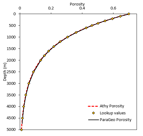
7.Validate the material characterisation by running a drained consolidation model. This is provided in the datafile Mat_001c_Case01a_cons.dat where gravity is slowly applied to a sediment column and is allowed to compact. Open the results corresponding to the last plot file in ParaView and perform a Plot Over Line in the centre of the column. Export the results in CSV format and copy/paste them in "Consolidation" sheet cell CH1 (including headers). Now you can visualize your predicted porosity curve compared to the target curve in the graph located at cell B26.
Comparison of target porosity curve (red discontinuous curve) with modelled curve (black curve). The diamond markers indicate the values extracted with the lookup table used to input the hardening table.
|
| Exercise (Mat_001c_Case01b) |
In the folder Mat_001c/Case01/Exercise/Data the data required to perform this exercise is provided. The proposed exercise corresponds to repeat the material characterisation and validation procedure for an Athy sandstone compaction trend with a depositional porosity of Ø0=0.41 and a compressibility of k=0.31 km-1. The values for Poisson's ratio and hardening law are provided in the .mat file
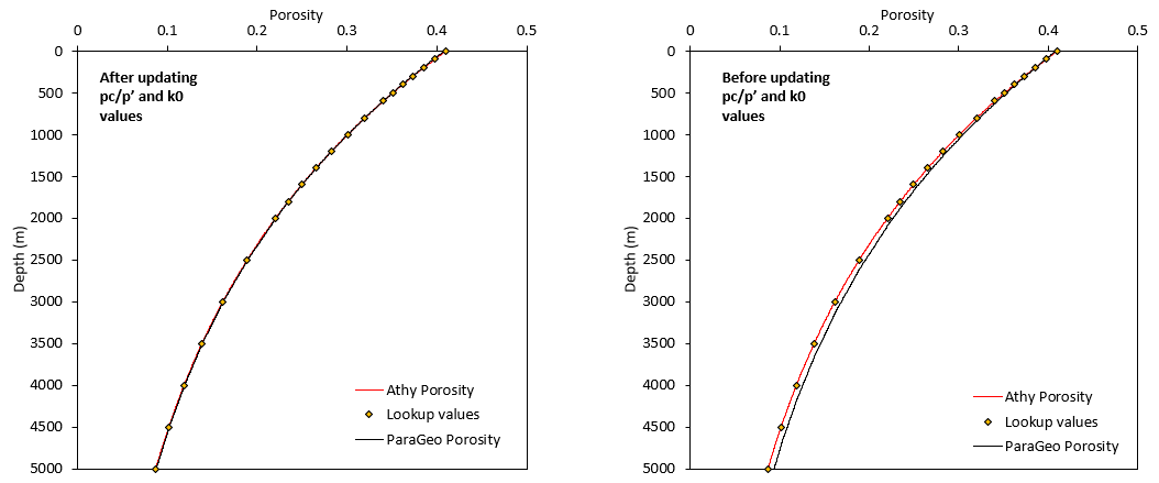
The results are provided in Mat_001c/Case01/Exercise/Results. See below the target Athy curve compared to the predicted/modelled compaction curves before and after updating the pc/p' and k0 values and updating the hardening table accordingly. Note that the results using the initial guess values show some deviation from the target curve.
Comparison of the modelled compaction curve with the target data. On the left the modelled results after updating the pc/p' and k0 values and correcting the hardening table. On the right the modelled results are obtained using the initial guess values.
|
References
Hantschel T. & Kauerauf, A. (2009) Fundamentals of Basin and Petroleum Systems Modeling. Springer-Verlag. Berlin Heidelberg 2009.
|

