The data files for the present tutorial case are in ParaGeo_Tutorial_Examples/Mat_004/Case02/Data and the spreadsheets with the results in ParaGeo_Tutorial_Examples/Mat_004/Case02/Results

 

In this tutorial case the behaviour of the power law with accelerated creep for high q model will be discussed. As shown in the overview section the rate of creep is described by the following equation:

 

 

As can be seen the equation is similar to the simple power law model but adding an extra term to account for the effect of deviatoric stress (q) in the creep strain rate. Hence this tutorial case builds from previous case (Case01 Power law model) and only the key differences with the previous model will be discussed.

 

The creep law data corresponding to Case02b is discussed below. It should be noted that the rest of the data is identical to previous tutorial case.

 

 

 

 

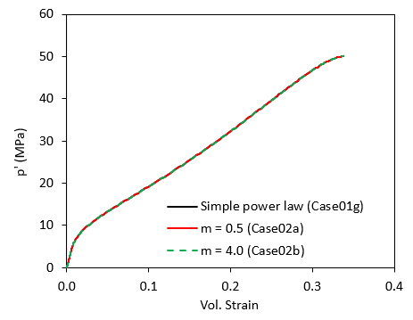
In the figure below the results for different hydrostatic compression test simulations (hct) are compared. A simulation using the simple power law model is compared to two simulations characterised with the accelerated creep for q model with different values of the mc exponent. As can be seen, because in a hct test the loading path follows the hydrostatic stress axis (q = 0) the solutions are identical to the simple power law model.

 

Comparison of the solution in hct simulations obtained from the simple power law model and two cases using the accelerated creep for high q model with different values for material parameter mc

 

 

 

To demonstrate the implications of using this model a series of confined triaxial tests simulations will be discussed. Such simulations consider three stages comprising:

 

1.A confining stage in which the sample is hydrostatically loaded (100 hours)

2.A triaxial loading stage in which confining pressure is held constant while an axial displacement is applied (20 hours)

3.A relaxation stage in which both the confining pressure and axial displacement are held constant (120 hours)

 

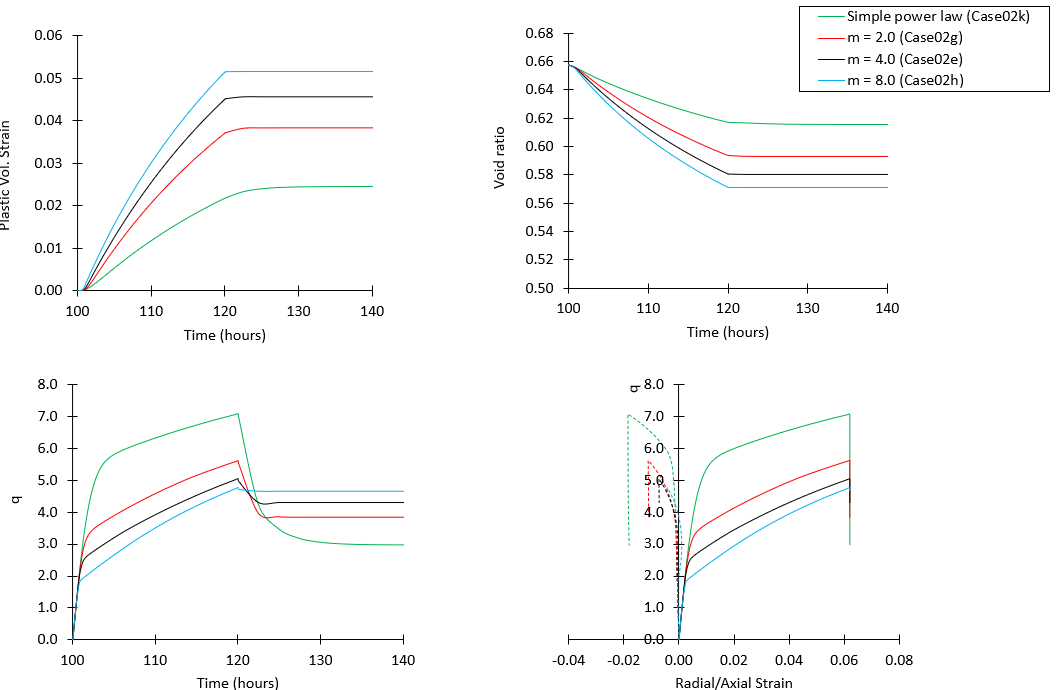
The results for 4 cases with different values of the exponent mc including a case with the material characterised with the simple power law model are shown in the figures below.

 

As can be observed the extra term results in additional plastic volumetric strain and therefore a lager void ratio reduction compared to the simple power law model due to the additional strain rate. When the triaxial loading stops both plastic volumetric strain and void ratio remain on an almost constant value. This is because in the present simulation the axial displacement is held constant during the holding period as opposed to the axial stress. Consequently during the hold period a stress relaxation is expected as opposed to further strain development due to creep. This is observed in the bottom left figure where there is a drop in deviatoric stress due to a drop in the axial stress (while radial stress is held constant). An interesting observation from the bottom left figure is that for different values of mc, different maximum/peak q values are reached, and the higher the peak q value, the larger the subsequent stress drop. For high values of mc the creep strain rate is increased and therefore more plastic creep strain develops during the loading phase relative to cases with low values of mc  what partially dissipates stress increase (stress increases due to the "locked" creep strain). This may explain the larger q values reached for cases with low mc values (with the limit case of the simple power law model). Then the larger drop in stress for cases with low mc may be explained because:

1.The actual yield surface is relatively small compared to cases with high mc value due to the lower plastic creep strain (e.g. actual pc is 4.89 MPa in case02k vs 5.18 MPa in case02h)

2.The apparent yield surface is relatively large compared to cases with high mc value due to the larger stresses developed

3.Thus, both previous points result on a higher distance between the actual and the apparent yield surface for cases with low mc compared to cases with high values requiring a larger stress drop for the stress path to return on the actual yield surface.

 

 

 

CTC test simulation results for several cases with different values of the mc exponent. Note that the time axis displays only a selected range.

 

 

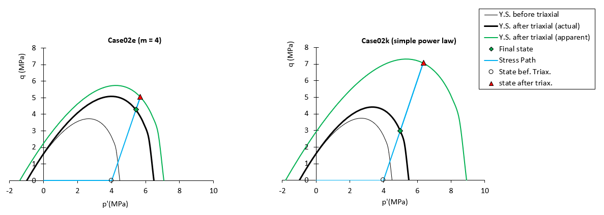
In order to support the previous observations the stress path and the yield surfaces at key selected times for case02e (m = 4) and case02k (simple power law) are shown in the figure below. In such figure it can be seen:

 

1.The actual yield surface size after triaxial loading for case02e is larger than in case02k because of the extra creep strain attributed to the accelerated creep with q

2.The apparent yield surface size for case02k is larger than in case02e because in the former case more portion of the axial strain imposed during triaxial loading is accommodated by stress increase due to the lower creep strain relative to case02e

3.For both cases when the triaxial loading terminates the stress path returns to the actual yield surface following the opposite direction of the triaxial loading path (from the red triangle to the green diamond). The length of such relaxation path is determined by the size ratio between the apparent and the actual yield surface and hence there will be a larger stress drop as such ratio increases.

 

Stress path and key yield surfaces and stress states at selected times for case02e (left) and case02k (right)

 

 

 

The table below compiling all the cases simulated and discussed in the present tutorial case is provided for reference purposes.

 

 

Table summarising model parameters and conditions for all the cases discussed in the present tutorial case