Case 1B Scaling Time for 100 Steps
The objective in this case is to achieve a quasi-static solution. This necessitates:
1Increasing the natural frequency of the system; i.e. allowing the stress applied at the top of the model to propagate more quickly through the model. Increasing the natural frequency lowers the critical time step and therefore increases the number of time steps within the time range 0.0 < t , 2.0.
2Ensuring that the frequency of loading is as low as possible; i.e. applying smooth load functions, to minimize dynamic deformation induced by changes in load.
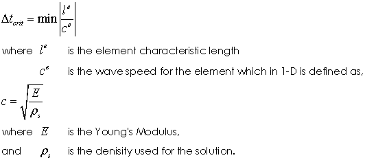
The critical time step is dependent on both the material properties and the size of the elements and for 1-D wave propagation is defined as:

By Default the mass-scaling constant, fmass = 1.0 so that ρs = ρ. Based on this value the critical time step in Case 1A is Δtcrit = 0.83 so that Δt = fcritΔtcrit = 0.58 and only four steps are required to reach the termination time t=2.0. In quasi-static problems, mass-scaling can be used to increase the natural frequency, and therefore reduce the critical time step. Note that mass-scaling scales the mass used to compute the dynamic solution, but does not affect loading (i.e. gravity loads).
The objective is to set the target time step and load ramp data such that the dynamic response is minimized and an approximately quasi-static response is predicted. In this first case the target time step is set to give approximately 100 steps for ramp time (1.0) defined for load case 1.
In ParaGeo the required mass-scaling for all elements in the domain so that fcritΔtcrit = Δttarg is automatically calculated based on a defined "Optimal time step". This is a straightforward method to define mass scaling and is generally recommended.
The data file for this exercise is located in directory: mech_001\Exercises\Case1B\Data. Look for ! TODO text in the datafile and follow the instructions.
Time_scaling_factors
The Time_scaling_factors data structure is added to the data file.
Data File |
|
* Time_scaling_factors ! --------------------------------- Optimal_time_step 1.0E-2
|
The target optimal time step is set to 0.01 so that approximately 100 steps will be used to simulate the load ramp time of 1.0. |
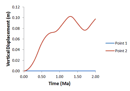
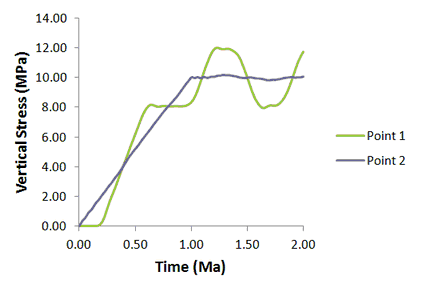
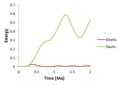
The results are visualized by plotting the high definition history data for global energy and points output in files mech_001_2d_Case1b_000.hdh and mech_001_2d_Case1b_001.hdh respectively. This data can be pasted into excel workbook mech_001.xls. Note that as the history files are comma delimited the Excel data import must be modified via Data->Text to Columns->Delimited->Comma.

As the surface load is a linear ramp between t=0.0 and t=1.0 the target quasi-static solution is linearly increasing displacement between t=0.0 and t=1.0 followed by constant displacement. The displacement for point 2, corresponding to the top of the column, however, exhibits a strongly dynamic response between time 1.0 and 2.0.

The dynamic response is also evident from the evolution of stress. The vertical stress at the base of the column remains almost zero until ca. t=0.2 and then subsequently overshoots the vertical stress at point 1 at ca. t=0.6. The delay is due to the time taken for the stress wave to arrive at the base of the column. The oscillatory response between time 1.0 and 2.0 is also evident.

Similarly, the global energy exhibits a low frequency oscillatory response between time 1.0 and 2.0.
Target_number_time_steps
Another alternative method generally recommended to define the simulation time step is definition of Target_number_time_steps keyword within * Control_data structure. This method has been more recently implemented in ParaGeo and it is specially advantageous for cases in which there are several simulation stages with very different durations and the objective is to use the same number of time steps per stage (and hence optimize the computation time). The advantages of using Target_number_time_steps instead of Optimal_time_step method for such mentioned cases are:
1.The number of time steps is directly specified so is more straightforward (no need to compute the corresponding time step size).
2.It minimizes dynamic effects upon the contrast of very different time step sizes when changing stages. Note that for a case with stages with very different durations, if Optimal_time_step method is used and the same number of time steps per stage is targeted, the Optimal_time_step needs to be re-specified at every stage. Thus mass-scaling changes at every stage and dynamic effects may be introduced. Note that with the Target_number_time_steps method mass-scaling does not change.
Note that for the present case the results are identical for both methods if the values are set consistently (i.e. same number of time steps are used to solve the problem by both methods). The datafile mech_001_2d_Case1b2.dat is provided as an example of usage of such method.
Data File |
|
* Control_data ! --------------------------------- Control_title "Stage 1" Solution_algorithm 1 Factor_critical_time_step 0.7 Maximum_number_time_steps 1000000 Target_number_time_steps 213 Termination_time 2.0 Output_frequency_plotfile -1 Output_time_plotfile 0.05 Screen_message_frequency 500
|
The target number of time steps is set to 213 so the same number of time steps as in the case defined with an Optimal_time_step of 1E-2 are used. |
Check the number of time steps used for the simulation in the .res file
The mech_001_2d_Case1b.res is a file output during the simulation in which a log of the operations performed is written. It provides useful information for debugging issues, detecting mistakes in the datafile, etc. In addition it provides useful information at the end of each control stage such as the number of time steps used up to that time and some CPU statistics. We can see the number of time steps used as shown below:
.res File |
|
Mechanical (Geomechanical) Analysis =================================== Number of control steps = 1 Total (Process) time = 2.00000 Number of mechanical time steps = 213
|
We can check that: 1.The current example considered only one stage (Number of control steps) 2.The simulation time is 2 time units 3.The current simulation has been run with 213 time steps |
| Key points |
1.In order to minimize dynamics/oscillation in the solution you should make sure to use enough mechanical time steps to solve the loads applied at each simulation stage. In such a way the load increment for each mechanical time step will be sufficiently low that the resulting inertia effects will be rather small. This is achieved by defining either the Target_number_time_steps in Control_data or defining the target time step size via Optimal_time_step keyword within Time_scaling_factors data structure. In both cases the code will automatically apply the corresponding mass-scaling required for each group in the simulation. Note that definition of Factor_critical_time_step < 1.0 in Control_data is also required (recommended default values are 0.9 in 2D problems and 0.7 in 3D problems).
2.The required number of time steps per simulation stage/load application is case dependent and depends on several factors (e.g. magnitude of the load applied, stiffness of materials, etc.). Nonetheless a good starting point is to use at least 10000 time steps per stage. For simulations coupling the mechanical and flow fields the number of mechanical steps per flow steps is also relevant to ensure stability. A minimum of 100 mechanical steps per flow step is recommended (but more may be required).
|
