Case01b CO2 Injection in Saline Aquifer (transient thermal)

Contents
The current case is identical to Case01a except that the transient thermal field will be solved by Pflotran-OGS in addition to the multiphase flow. Therefore only key differences in data required to run a simulation solving the thermal field will be discussed in detail here. It is assumed that the user has previously undertaken Case01a.
The files for the current case are provided in PFO_001\Case01b\Data. These comprise:
•PFO_001_CASE01B.dat input data file for the geomechanical model (ParaGeo)
•PFO_001_CASE01B.in input data file for the flow model (Pflotran-OGS)
•fluid_data: folder containing data files for CO2 equation of state database and saturation functions which are required for the flow simulation in Pflotran-OGS. These are the same files as in the previous case Case01.
•grdecl_data: folder containing the grid data for the flow model previously generated in Case01 Grid Generation.
Note that the folder structure and the files included are the same as in the previous case.
Pflotran input data (PFO_001_CASE01B.in)
Here the key data within the PFO_001_CASE01B.in file which differs from Case01a in order to solve for a transient thermal field is described. Note that for specific details on each of the keywords / cards the user is referenced to the official Pflotran-OGS web page.
Simulation Block
Material properties
Some additional material properties to Case01a need to be defined in order to solve the thermal field.
Boundary conditions
In the current case, in addition to the AQUIFER_DATA which provides pressure support, thermal boundary conditions are defined for the top and bottom surfaces of the reservoir with a prescribed temperature consistent with the value obtained from the initial temperature gradient applied in EQUILIBRATION.
Wells
Additional cards are required in WELL_DATA to characterize the enthalpy of the injected fluid.
|
ParaGeo input data (PFO_001_CASE01B.dat)
The ParaGeo input file is almost identical to the one used in Case01a. The only difference is the need to set the Thermal_field_flag keyword to 1 within Pflotran_coupling_data in order to couple the thermal field.
|
Results
Flow model ResInsight Results
The results discussed here are provided in PFO_001\Case01b\Results.
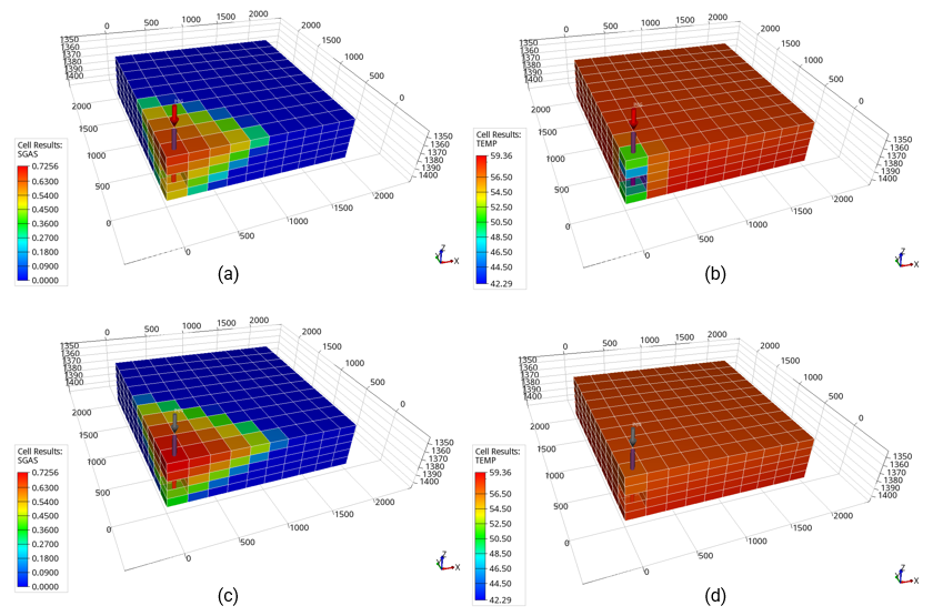
The figure below shows gas saturation and temperature contours at the end of the injection period (20 years) and 29 years after the injection has ceased. It can be observed that:
i.Gas saturation in the well cells has decreased over time after the injection has ceased and gas has spread over a wider volume (e.g. see the 6th cell in the X axis).
ii.The decrease in temperature due to CO2 injection occurs mainly at the well and adjacent cells. This may be likely strongly controlled by the boundary conditions of prescribed temperature at the top and bottom surfaces of the reservoir.
Gas saturation (left) and temperature (right) distribution within the reservoir after 20 years of injection (a, b) and at the end of simulation, 29 years after injection has ceased (c, d)
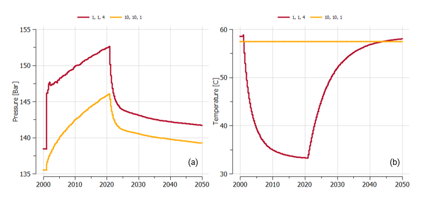
The summary plots below show the evolution of pressure and temperature in two cells for which summary output is requested. The two cells correspond to a well cell (1,1,4) and a cell located in the opposite corner of the reservoir (10,10,1). It is noted that the well cell is located 30 m deeper than the cell in the opposite corner (thus influencing the initial pressure and temperature values). In the plots it can be seen that:
i.The temperature in the well cell has almost recovered its initial temperature
ii.The temperature in the opposite corner of the reservoir is undisturbed, in agreement with the observations made on the contour plots
iii.The pressure increase due to injection affects the whole reservoir, but it is more pronounced near the well, reaching pressure magnitudes of ~153 Bar, whereas in the opposite corner cell the maximum pressure reached is ~146 Bar.
Evolution of pore pressure and temperature in a well cell (red curve) and in a cell in the opposite corner (orange curve)
Geomechanical model ParaView results
The results discussed here are provided in PFO_001\Case01b\Results\PFO_001_CASE01B_parageo_results.
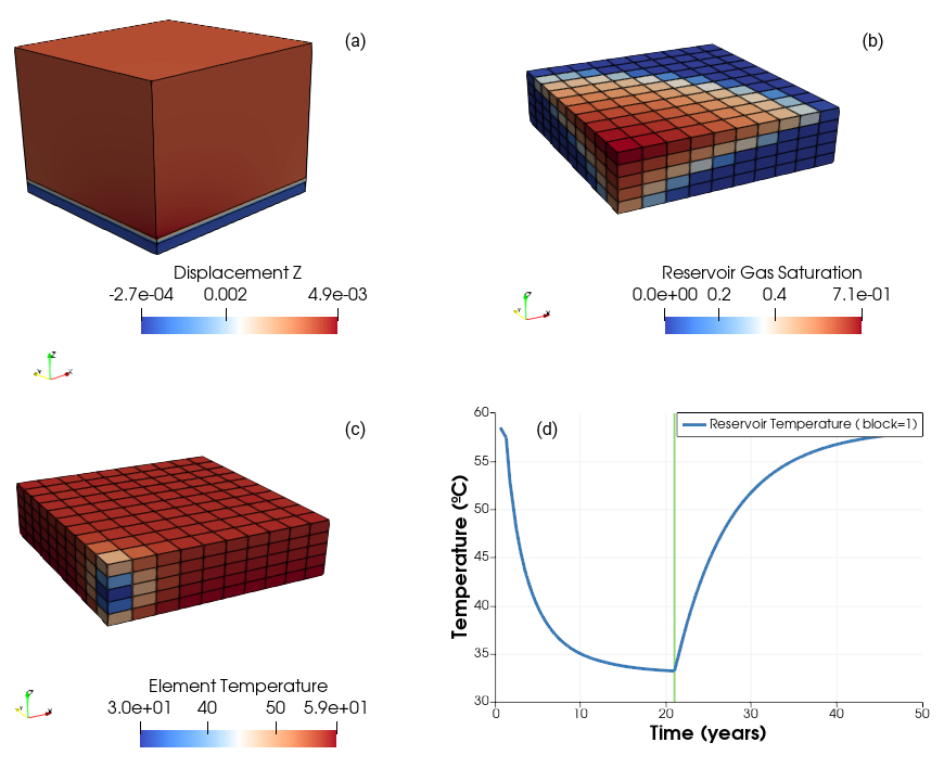
The figure below shows several contour plots after 20 years of injection. Note how the results output by ParaGeo also incorporate the state variables from the Pflotran-OGS (figures b and d) and figure (d) shows the evolution of temperature for the same cell that was output as a summary in Pflotran-OGS.
Vertical displacement (a), Reservoir gas saturation (b) and element temperature (c) distribution after 20 years of injection. Reservoir temperature evolution in a well cell (d). Figure (a) shows all the formations whereas figures (b) and (c) show the reservoir with V.E. = 10.
|