Case01a CO2 Injection in Saline Aquifer (isothermal case)

Contents

IMPORTANT NOTES

•For simulations in which results are going to be exported in an eclipse grid format to be loaded in ResInsight it is compulsory to use capital letters only to define the file name in order that the results are also output using capital letters only.

•The ResInsight version used to generate the plots is 2022.06.0. It is noted that the latest versions (e.g. 2024.12.0) may not be compatible with the summary data exported from Pflotran-OGS into the .UNSMRY and .SMSPEC files.

The files for the current case are provided in PFO_001\Case01a\Data. These comprise:

•PFO_001_CASE01A.dat input data file for the geomechanical model (ParaGeo)

•PFO_001_CASE01A.in input data file for the flow model (Pflotran-OGS)

•fluid_data: folder containing data files for CO2 equation of state database and saturation functions which are required for the flow simulation in Pflotran-OGS. The files include:

▪co2_dbase.dat : Database to describe the CO2 equation of state

▪SGFN_psi.dat: Gas saturation function

▪SWFN_psi.dat: Water saturation function

•grdecl_data: folder containing the grid data for the flow model previously generated in Case01 Grid Generation.

Note that to run a coupled simulation all the previous listed files and folders need to be in place. The ParaGeo file name as well as the files within the fluid_data and grdecl_data folders are referenced within the Pflotran-OGS file. To run the coupled simulation the Pflotran-OGS file must be run in a DOS command prompt by executing the following command:

C:\...\PFO_001\Case01a\Data>pflotran_ogs -input_prefix PFO_001_CASE01A_STEP02

Pflotran input data (PFO_001_CASE01A.in)

In Pflotran and Pflotran-OGS the input data is defined via the so-called "cards" (which would be the equivalent of ParaGeo keywords) and those cards may belong to "blocks" or "card blocks" (the equivalent of ParaGeo data structures). These card blocks may have several sub-levels (e.g. a given card may have different input options to choose from). Each sub-level of card blocks ends with either "/" or an "END". It is good practice to apply different indentation levels for every card sub-level so that the data in the data file becomes easier to read. Here in the manual we highlight the start and end of every sub-level of card block in a different color in order to facilitate a quick identification of the different levels.

Below the data within the PFO_001_CASE01A.in file is described. Note that for specific details of each of the keywords / cards the user is referenced to the official Pflotran-OGS web page.

Simulation Block

Data File

SIMULATION

SIMULATION_TYPE SUBSURFACE

PROCESS_MODELS

SUBSURFACE_FLOW Flow

MODE GAS_WATER

OPTIONS

ISOTHERMAL

RESERVOIR_DEFAULTS

GEOMECHANICS_EXTERNAL

DATA_FILE PFO_001_CASE01A.dat

TRANSFER_METHOD memory

END

•SIMULATION_TYPE is set as SUBSURFACE (compulsory for CO2 applications).

•In PROCESS_MODELS the SUBSURFACE_FLOW and GEOMECHANICS_EXTERNAL are selected.

•GEOMECHANICS_EXTERNAL is compulsory to couple to ParaGeo. Two child keywords are used:

▪DATA_FILE defining the geomechanical model file name.

▪TRANSFER_METHOD defining the method for transferring the data between ParaGeo and Pflotran (i.e. memory or file based transfer of data).

Import of Grid

Here the import of grids to define both the model mesh and cell material properties is defined.

Data File

GRID

TYPE grdecl grdecl_data/PFO_001_Case01_header.grdecl

END

•Using the GRID keyword we define:

▪The TYPE of format used to define the input grid (grdecl in this case).

▪The file name (and path) for the header file exported in Case01 Grid Generation.

The header file content exported in Case01 Grid Generation is shown below:

Data File (PFO_001_Case01_header.grdecl)

dimens

10 10 5

external_file PFO_001_Case01_coord.grdecl

external_file PFO_001_Case01_PERMX.grdecl

external_file PFO_001_Case01_PERMY.grdecl

external_file PFO_001_Case01_PERMZ.grdecl

external_file PFO_001_Case01_PORO.grdecl

•The file contains:

▪dimens keyword defining number of cells in X, Y and Z.

▪links to all external files containing input data (grid coordinates and material properties).

Simulation time and Time step data

Data File

TIME

FINAL_TIME 50 y

INITIAL_TIMESTEP_SIZE .005 y

MINIMUM_TIMESTEP_SIZE 1.0D-10 y

MAXIMUM_TIMESTEP_SIZE .25 y at 0 y

END

•The times are defined in years (y).

Output options

Data File

OUTPUT

MASS_BALANCE_FILE

PERIODIC TIMESTEP 1

END

SNAPSHOT_FILE

PERIODIC TIME 1.0 y

WRITE_DENSITY

WRITE_VISCOSITY

VARIABLES

TEMPERATURE

GAS_SATURATION

(...)

MINERAL_POROSITY

END

FORMAT HDF5 SINGLE_FILE

END

PRINT_PRIMAL_GRID

ECLIPSE_FILE

PERIODIC TIME 1.0 y

PERIOD_SUM TIMESTEP 1

OUTFILE

WRITE_DENSITY

WRITE_VISCOSITY

SUMMARY_D

BPR 1 1 4

BGSAT 1 1 4

(...)

BTEMP 10 10 1

END_SUMMARY_D

END

LINEREPT

END

•In OUTPUT keyword the options for output from Pflotran-OGS are defined. These include:

▪The type of files / data being output (e.g. mass balance, summary, snapshot, etc).

▪The variables being output.

▪The output frequency.

•SNAPSHOT_FILE request output of results in hdf5 format for visualisation in ParaView.

•ECLIPSE_FILE requests output of results in Eclipse format for visualisation in ResInsight. In addition to the plot files, output of summary files for selected variables in selected cells is requested (listed within SUMMARY_D keyword). In the present case these summary outputs correspond to one cell where injection is performed (where well is defined) and a cell located in the opposite corner at the top of the reservoir.

Material properties

Pflotran-OGS provides several compressibility functions to define the material properties. For ParaGeo-Pflotran two-way coupled simulations it is compulsory to use a new implemented function which is called GEOMECH. This function uses the initial pore pressure defined from geostatic initialisation as the reference pressure, whereas the magnitude of the rock compressibility is computed in ParaGeo from the poroelastic material properties.

Data File

MATERIAL_PROPERTY formation

ID 1

ROCK_COMPRESSIBILITY_FUNCTION GEOMECH

ROCK_REFERENCE_PRESSURE INITIAL_PRESSURE

CHARACTERISTIC_CURVES ch1

•A single material property is defined.

•Note that parameters such as porosity and permeability are not defined here because they are input via the eclipse grids exported from ParaGeo, allowing for spatial distribution of the properties in different cells (even though in the present case the properties are homogeneous across the whole reservoir).

•The compulsory compressibility function for two-way ParaGeo-Pflotran coupled simulations is used by defining ROCK_COMPRESSIBILITY_FUNCTION with the option GEOMECH.

•For the GEOMECH compressibility function it is compulsory to define ROCK_REFERENCE_PRESSURE with the option INITIAL_PRESSURE.

Saturation functions

Data File

CHARACTERISTIC_CURVES ch1

TABLE swfn_table

PRESSURE_UNITS psi

external_file fluid_data/SWFN_psi.dat

END

TABLE sgfn_table

PRESSURE_UNITS psi

external_file fluid_data/SGFN_psi.dat

END

•The saturation functions are imported from the SWFN (water) and SGFN tables defined in files within the fluid_data folder.

•The pressure unit used to define the values in those tables needs to be specified (psi in the present case).

•The SWFN_psi.dat file contains three columns defining:

▪C1: Water saturation (Sw)

▪C2: Relative permeability of water (Krw)

▪C3: Water-Gas capillary pressure (PCwg)

•The SGFN_psi.dat file contains three columns defining:

▪C1: Gas saturation (Sg)

▪C2: Relative permeability of gas (Krg)

▪C3: Oil-Gas capillary pressure (PCog)

Fluid properties

Fluid properties and the equations of state (EOS) for each fluid (water and CO2 gas) need to be defined.

Data File

FLUID_PROPERTY

PHASE LIQUID

DIFFUSION_COEFFICIENT 2.0d-9

FLUID_PROPERTY

PHASE GAS

DIFFUSION_COEFFICIENT 2.0d-5

BRINE 0.001 MOLAL

EOS WATER

SURFACE_DENSITY 1000.0 kg/m^3

END

EOS GAS

SURFACE_DENSITY 1.0 kg/m^3

CO2_DATABASE fluid_data/co2_dbase.dat

END

•Default EOS are used where the CO2 behaviour is defined via a table provided within the fluid_data folder.

Equilibration

Equilibration is used to define the initial state of the reservoir before any production / injection is performed.

Data File

EQUILIBRATION

PRESSURE 13.5 MPa

DATUM_D 1350 m

TEMPERATURE_TABLE

D_UNITS m

TEMPERATURE_UNITS C

RTEMPVD

0.0 10.0

1500.0 62.5

END

•The initial pressure in the reservoir is defined as 13.5 MPa at a datum of 1350 m. All the cells in the reservoir will be applied an initial pressure value following a hydrostatic gradient.

•The initial temperature distribution is defined via a table based on a surface temperature of 10 ºC and a temperature gradient of 0.035 ºC / m. This is achieved by defining:

▪10 ºC at 0 m depth

▪62.5 ºC at 1500 m depth

•Note that TEMPERATURE_UNITS must be compulsorily defined as C (degrees celcius).

Aquifers

AQUIFER_DATA may be used to define analytical aquifer boundary conditions that may be assigned to any reservoir boundary to provide pressure support. The aquifer will then act as a sink (if reservoir pressure increases) or as a pressure source (if reservoir pressure drops) in response to pressure changes within the reservoir allowing flow in and out of the boundary, thus stabilizing the reservoir pressure during the simulation.

Data File

AQUIFER_DATA north

BACKFLOW

DEPTH 1375.0 m

THICKNESS 50 m

WIDTH 20000 m

PERM 300.02331 mD

COMPRESSIBILITY 2.38E-10 1/Pa

POROSITY 0.3

VISCOSITY 1 cP

CONN_D 1 10 10 10 1 5 Y+

END

AQUIFER_DATA east

(...)

CONN_D 10 10 1 10 1 5 X+

END

•Two AQUIFER_DATA are defined, one that will be assigned to the north boundary and another that will be assigned to the east boundary.

•The material properties for the analytical aquifers are defined so that they match the material properties for the reservoir.

•In the current case, the WIDTH is defined large enough to ensure that there is no excessive pressure build up for the considered target CO2 injection rate, volume and reservoir model dimensions.

•CONN_D defines the cells to which each analytical aquifer is connected. This is defined by providing the connected cells indexes as Imin Imax Jmin Jmax Kmin Kmax. The Y+ and X+ specified at the end of the indexes in both aquifers are used to identify the cell faces to which connection between the reservoir and the aquifer is established (e.g. X+ indicates that the connected cell face is the one that would be shared by cells Imax with (Imax+1).

Wells

WELL_DATA is used to define well boundary conditions to perform injection and / or production. This is done by defining for the cells representing the well, the injection / production conditions with the time periods when the well is open or shut.

Data File

WELL_DATA injg

CIJK_D 1 1 3 4

WELL_TYPE GAS_INJECTOR

THETA_FRACTION 0.25

BHPL 25 MPa

SHUT

TIME 1 y

OPEN

TARG_GM 0.25 Mt/year

TIME 21 y

SHUT

END

•The wells in Pflotran-OGS are vertical and hence in CIJK_D the input indices correspond to I J Kmin Kmax

•Because the model considers quarter symmetry two considerations have to be taken into account:

▪The injection rate is scaled by 1/4, so that TARG_GM is input as 0.25 Mt/year to consider 1 Mt/year.

▪THETA_FRACTION is defined with a factor of 0.25 which establishes the well cell connections.

•In the current case, the well is:

▪SHUT until t = 1 year.

▪OPEN from t = 1 year to t = 21 years.

▪SHUT from t = 21 years onwards.

ParaGeo input data (PFO_001_CASE01A.dat)

Here the key data concerned with the ParaGeo-Pflotran-OGS coupled simulations in the PFO_001_CASE01A.dat file is discussed. Note that the geometry and mesh data for the geomechanical model (ParaGeo) are the same as those used during the export of the flow model (Pflotran-OGS) grid. Note also that the geomechanical model considers two initialisation stages prior to performing the coupled simulation stage (the control data for this is discussed below).

Material data

Two material data structures are defined; the Reservoir and Shale material properties; the latter assigned to overburden and underburden. Note that material assignment is done within Group_data (not discussed here).

Data File

* Material_data NUM=1

! ---------------------------------

Name "Reservoir"

! ----------------------------------------------

Grain_stiffness 70000E6 ! Pa

Grain_density 2700.00 ! Kg/m3

! ----------------------------------------------

Porosity 0.300

! ----------------------------------------------

Elastic_model_type 1

Elastic_properties IDM=2

/Young's Modulus (E)/ 12600.0E6

/Poisson's Ratio (V)/ 0.2

! ----------------------------------------------

Fluid_saturation 1.0

Singlephase_fluid 1

! ----------------------------------------------

Permeability_type 2

Permeability_vs_porosity IDM=19 JDM=2

/Porosity/

0.010 0.025 ... 0.800

/Perm mD/

0.101324997 0.101324997 ... 202.6499932

* Material_data NUM=2

! ---------------------------------

Name "Shale"

! ----------------------------------------------

Grain_stiffness 70000E6 ! Pa

Grain_density 2700.00 ! Kg/m3

! ----------------------------------------------

Porosity 0.100

! ----------------------------------------------

Elastic_model_type 1

Elastic_properties IDM=2

/Young's Modulus (E)/ 7200.0E6

/Poisson's Ratio (V)/ 0.3000

! ----------------------------------------------

Fluid_saturation 1.0

Singlephase_fluid 1

! ----------------------------------------------

Permeability_type 1

Permeability 5.0E-19

•The porosity and the elastic properties are used to calculate the reference reservoir compressibility as:

PFO_001_eq_01

where cp is the compressibility, ʋ is the Poisson's ratio, Øeff is the reservoir effective porosity and E is the reservoir Young's modulus. Note that as we are using the GEOMECH compressibility function in Pflotran-OGS the reservoir effective porosity is calculated as:

where Ø0 is the reservoir initial effective porosity, pt is the pore pressure at the current time step and pt-1 is the pore pressure at the previous time step.

•Note that in the ParaGeo data file (geomechanical model) a single-phase fluid is assigned to the materials but in the actual flow simulation (performed by Pflotran-OGS) multiphase flow is considered.

•The Permeability_type set to 2 uses a permeability vs porosity look-up table. Note that in ParaGeo-Pflotran simulations the permeability values defined are not directly used; but are used to calculate permeability multipliers upon a porosity change. For example:

▪Reference porosity is 0.3 which has a defined permeability value of 22.58 mD.

▪At time t, the reservoir porosity is 0.25 with a look-up perm value of 9.94 mD.

▪The calculated perm multiplier is then Kmult = 9.94 / 22.58 = 0.4402.

▪Then because the initial vertical and horizontal permeabilities (values at reference porosity) were defined with values of 30 mD and 300 mD respectively, the updated permeabilities at time t when the porosity is 0.25 are 13.21 mD (i.e. Kmult*30) and 132.06 mD (i.e. Kmult*300) respectively.

•Note that the permeability for the shale material is a dummy value as flow is not simulated within the overburden nor underburden.

Initial Conditions

The initial conditions in the geomechanical model are defined via a gravity loading (Gravity_data) and geostatic data (Geostatic_data). The latter also has assigned Spatial_variation_definition and Spatial_variation_values in order to define an initial temperature distribution. Whilst the temperature will not be relevant for geomechanics in the current case (as there are no temperature-dependent processes included in the constitutive models) it is defined for plotting purposes; the reservoir temperature will be provided by Pflotran-OGS and we prescribe temperature distribution in the overburden and underburden from the geomechanical model (thus avoiding zero temperature values in the plots).

Data File

* Geostatic_data NUM=1

! ---------------------------------

Groups IDM=3

"deep_shale"

"reservoir"

"shallow_shale"

K_value_x 0.7

K_value_y 0.7

Pore_pressure_distribution "Hydrostatic"

Temperature_spatial 1

* Spatial_variation_definition NUM=1

! -----------------------------------------

Description "Temperature vs. Depth"

Type "Absolute"

Distribution "Depth_dependent"

Variation_assignment 1

* Spatial_variation_values NUM=1

! -----------------------------------------

Description "Temperature vs. Depth"

Time 0.0

Values_vs_depth IDM=2 JDM=2

/Depth/ 0.0 1500.0

/Value/ 10.0 62.5

* Gravity_data

! ----------------------------------------

Gravity_constant 9.81000

Time_curve "Step_ramp"

•Geostatic_data for the 3 groups in the geomechanical model is defined.

•The initial pore pressure distribution will be hydrostatic pressure.

•The initial vertical stress distribution will result from the response of the model to the applied gravity loading which is dependent on the material and fluid properties (densities and porosities) in the different formations.

•The initial horizontal stresses are defined to be a factor of the vertical stress at each cell by specifying the K_value_x and K_value_y keywords.

•The initial temperature distribution defined in Spatial_variation_values is consistent with the distribution defined in the Pflotran-OGS file.

It is noted that during gravity loading, the model will develop vertical compressional strains which will result in vertical subsidence. In order to enhance the match between the Pflotran-OGS and ParaGeo initial coordinates for the reservoir cells, a secondary geostatic stage is performed where displacements and coordinates will be reset back to zero. This is achieved by defining appropriate keywords within Geostatic_control_data for each stage.

Data File

* Geostatic_control_data

! ---------------------------------

Description "Apply_Gravity_Load"

Stress_constitutive_model "Standard"

Stress_initialisation_type "Standard"

Displacement_reinit_flag 0

State_reinit_flag 0

Time_curve "Step_ramp"

* Control_data

! ================================================

Control_title "Geostatic"

* Geostatic_control_data

! ---------------------------------

Displacement_reinit_flag 3

* Control_data

! ================================================

Control_title "Disp_reinit"

.....

•A Geostatic_control_data is defined for each of the two initialisation stages (note that Control_data in ParaGeo defines the end of a simulation stage).

•In the first stage where gravity initialisation is applied, default options are defined.

•In the second stage Displacement_reinit_flag is set to 3. This will:

i.Save the previously calculated stress distributions and ramp them up from zero over the new stage (the gravity loading will be re-applied as well).

ii.At the start of the stage, reset the mesh coordinates back to their original location as well as the displacement state variables.

iii.At the end of the stage, after plot file output, reset again the displacement state variable.

•Note that here only the name (Control_title) of the data structures is shown, but more keywords defining stage duration, time steps, plot file output frequency, etc. are actually defined in the data file.

Pflotran coupling

In Pflotran_coupling_data the groups coupled with Pflotran-OGS and other coupling options are defined.

Data File

* Pflotran_coupling_data

! ---------------------------------

Groups IDM=1

"reservoir"

Coupling_method 1

Units_list IDM=4

"stress"

"length"

"temperature"

"density"

Units IDM=4

"Pa"

"m"

"Celsius"

"kg/m^3" !/

Output_level 2

•In the Groups keyword the groups that will be simulated in the flow model (and hence will be coupled) are listed. In the current case this consist of the reservoir group only.

•Coupling_method set to 1 defines a two-way coupled simulation (information is passed from Pflotran-OGS to ParaGeo and vice versa at each flow step).

•Units_list and Units keywords are used to define the units used in Pflotran-OGS for each physical quantity.

•Output_level is a keyword used to define the level of detail in the simulation log data output to the .res file. When set to 2 this provides a medium level of output.

Output data

ParaGeo by default exports the geomechanical model results in .hdf format plot files which may be visualised in ParaView. For exporting the geomechanical model results in an Eclipse grid format that may be visualised in ResInsight the Spatial_volume data structure is defined. Note that in the current case the results in the geomechanical model HEX mesh will be exported, however, the Spatial_volume data structure also allows the mapping and export of the results to an arbitrary user-defined grid.

Data File

* Spatial_volume

! ---------------------------------

Name "EGRID"

Output_flag 2

Eclipse_output_type "Unformatted"

•A name for the Spatial_volume is defined (compulsory).

•Output_flag set to 2 requests that both, standard .hdf plot files and Eclipse plot files are output.

Definition of stages

The geomechanical model considers 3 stages:

1.Geostatic initialisation with application of gravity.

2.Displacement reinitialisation (to recover the original geometry after any gravity-driven compaction has occurred).

3.Coupled simulation of injection with Pflotran-OGS.

As previously mentioned Control_data defines the end of a ParaGeo simulation stage. The stage where ParaGeo is coupled to Pflotran-OGS uses the definition of the Pflotran_control_data structure. Below, only the data defining the last stage (injection) is described in detail.

Data File

* Control_data

! =========================================

Control_title "Geostatic"

.....

* Control_data

! =========================================

Control_title "Disp_reinit"

.....

* Pflotran_control_data

! -----------------------------------

Control_title "Injection"

Target_number_timesteps 250

Screen_message_frequency 100

Output_time_plotfile 0.5

Output_frequency_plotfile -1

•Control_title defines a name for the stage.

•Target_number_timesteps defines the number of mechanical steps performed for each flow step.

•Screen_message_frequency set to 100 defines that the simulation information will be printed to the DOS window every 100 coupling steps.

•Plot files will be output:

▪every 0.5 years as defined by Output_time_plotfile set to 0.5.

▪at the end of simulation as defined by Output_frequency_plotfile set to -1.

Results

Description of result files

The results for the current case are provided in PFO_001\Case01a\Results. While results output from the flow model by Plotran-OGS are located in that folder, geomechanical model results output by ParaGeo are located in a sub folder PFO_001\Case01a\Results\PFO_001_CASE01A_parageo_results. Note that such sub-folder is automatically created during the simulation to keep the output from both codes separated.

The Plotran-OGS results include:

▪PFO_001_CASE01A.h5 main hdf plot file containing the results for all output time steps

▪PFO_001_CASE01A-nnn.xmf definition file for the plot output number nnn that may be loaded in ParaView for visualizing the results within the .h5 file

▪PFO_001_CASE01A-domain.h5 hdf file containing the grid topology

▪PFO_001_CASE01A.EGRID eclipse grid file that may be loaded in ResInsight

▪PFO_001_CASE01A.INIT file containing grid properties for the eclipse grid format results

▪PFO_001_CASE01A.SMSPEC index file containing metadata about the summary variables stored in the associated .UNSMRY file. This file may be loaded in ResInsight to obtain line plots

▪PFO_001_CASE01A.UNRST file containing the solution properties for the eclipse grid format results

▪PFO_001_CASE01A.UNSMRY summary file containing numerical results from which line graphs may be obtained in ResInsight. For that purpose the associated .SMSPEC must be loaded

▪PFO_001_CASE01A-mas.dat ASCII file containing mass balances at each simulated time step

The ParaGeo results include:

▪PFO_001_CASE01A.res log file containing details from the simulation

▪PFO_001_CASE01A_nnn.plt hdf plot file containing the results for the plot output number nnn

▪PFO_001_CASE01A_nnn.xmf definition file for the plot output number nnn that may be loaded in ParaView

▪PFO_001_CASE01A.xmf index .xmf file that may be loaded in ParaView to load all the plot file series at once (which allows forward and backward navigation of the simulated time)

▪PFO_001_CASE01A_geostatic.plt hdf plot file containing the results for the plot output number nnn corresponding to the geostatic initialisation stages (before any coupling to Pflotran-OGS is performed).

▪PFO_001_CASE01A_geostatic_nnn.xmf definition file for the plot output number nnn for the geostatic initialisation stages that may be loaded in ParaView

▪PFO_001_CASE01A_geostatic.xmf index .xmf file that may be loaded in ParaView to load all the plot file series for the geostatic initialisation stages at once

▪PFO_001_CASE01A_EGRID.EGRID eclipse grid file that may be loaded in ResInsight

▪PFO_001_CASE01A_EGRID.UNRST file containing the solution properties for the eclipse grid

▪Other files which are not provided such as .gmr or .sdg files containing geometry and grid plots respectively

Flow Model ResInsight Results

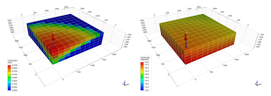
Here the results exported from Pflotran-OGS in an Eclipse grid format will be discussed. These are located in PFO_001\Case01a\Results. The PFO_001_CASE01A.EGRID is imported in ResInsight by clicking on the icon (or alternatively clicking on File/Import/Eclipse Cases/Import Eclipse Case) and browsing to the file. For comprehensive tutorials on ResInsight the user is referenced to ResInsight Tutorials.

The figure below shows the distribution of gas saturation and gas pressure within the reservoir at the end of injection.

PFO_001_Case01a_2

Gas saturation (left) and gas pressure (right) distributions within the reservoir after 20 years of injection

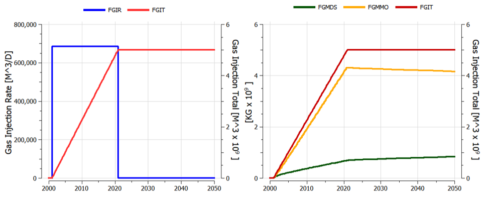
In the ResInsight plot editor, it is straightforward to construct plots relevant to a particular analysis by clicking on the icon to open the plot window and then clicking on the icon.

In the figure below, the left plot corresponds to the CO2 injection rate and total CO2 injected volume, whereas the right plot corresponds to the total amount of gas (FGIT), i.e. the amount of gas dissolved in brine (FGMDS) which increases over time even after injection stops and the mobile gas (FGMMO) which reduces after injection stops.

PFO_001_Case01a_3

The left figure shows CO2 injection rate (blue) and cumulative injected volume (red). The right figure shows Total injected CO2 (red), CO2 dissolved in brine (green) and mobile gas (orange)

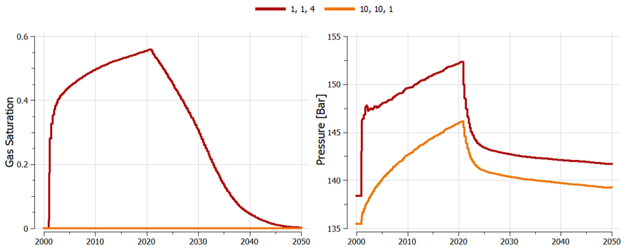
The summary plots requested in the Pflotran-OGS input file can be visualised in the ResInsight plot editor. The figure below shows the evolution of gas saturation and pressure for the two requested grid cells which correspond to a well cell (red line) and in a cell located in the opposite corner (orange line).

PFO_001_Case01a_4

Gas saturation (left) and pressure as a function of time in a well cell (red) and in a cell in the opposite corner (orange) within the reservoir

Geomechanical Model ResInsight Results

The geomechanical model results loadable in ResInsight are in PFO_001\Case01a\Results\PFO_001_CASE01A_parageo_results. Similar to the workflow for importing flow model results, we need to import the eclipse case by loading the corresponding .EGRID file.

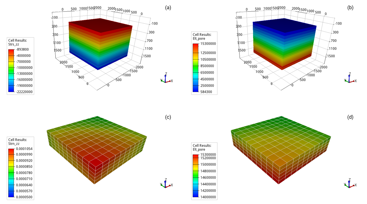
The figure below shows contour plot results for vertical stress, pore pressure and vertical strain after 20 years of injection. Plot (b) shows how the reservoir pressure has increased due to the simulated injection whereas the overburden and underburden show the initial hydrostatic pressure distribution because they are not coupled (flow is not solved for those formations). It can be seen as well that the increased pressure due to injection lead to a small vertical dilation within the reservoir, especially at the well location shown by the positive values reaching a maximum vertical strain magnitude of 0.0001054.

PFO_001_Case01a_5

Effective vertical stress (a), Pore pressure (b and d) and vertical strain (c) geomechanical model contour plots after 20 years of injection. Top plots show the complete geomechanical model domain encompassing the three formations whereas the bottom plots show only the reservoir cells with a V.E. = 10. Note that in stress and strain plots negative values indicate compression whereas positive values indicate extension (continuum mechanics sign criteria)

Geomechanical model ParaView results

Here the results from ParaGeo in hdf format loadable into ParaView are briefly discussed for demonstrative purposes on post-processing. These are located in PFO_001\Case01a\Results\PFO_001_CASE01A_parageo_results. Note that the Pflotran-OGS results output in hdf format which are loadable in ParaView are not discussed as they would be equivalent to the previously discussed ResInsight flow model results.

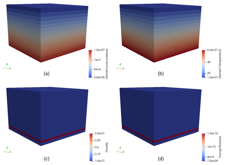
The initialisation results may be visualized by loading the PFO_001_Case01A_geostatic.xmf file into ParaView. These results are helpful in observing the model definition, materials, groups, pore pressure and temperature gradient at initial stage.

PFO_001_Case01a_6

Pore pressure (a) Temperature (b) Porosity (c) and Young's modulus (d) after initialization stage

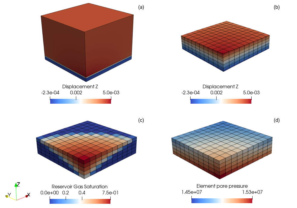
The simulation results may be visualized by loading the PFO_001_Case01A.xmf file into ParaView. Note that these results include output from both the geomechanical (ParaGeo) and flow model (Pflotran-OGS) where the state variables from the latter are preceded by "Reservoir" in the name (e.g. "Reservoir pore pressure" comes from Pflotran-OGS, "Element pore pressure" comes from ParaGeo).

PFO_001_Case01a_7

Vertical displacement (a and b), gas saturation (c) and pore pressure (d) after 20 years of injection. Plot (a) shows the complete domain whereas plots (b), (c) and (d) show the reservoir only. In plot (b) the mesh is deformed according to the displacement (warp by vector) with a magnification factor of 105 to the displacement magnitude. Plots (c and d) have V.E. = 10

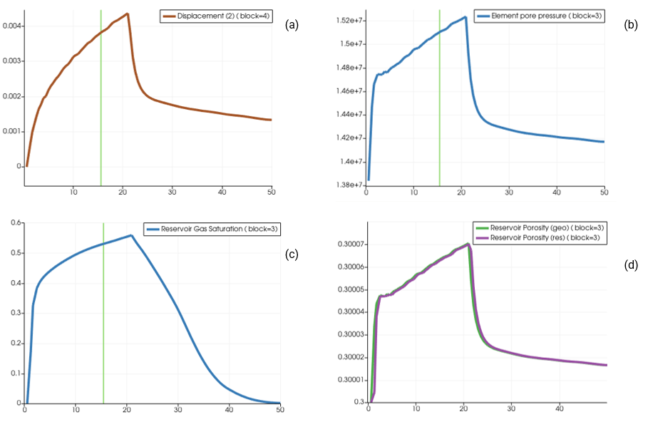
Note that in ParaView users may select an element (cell) or a node and perform a "Plot selection over time" filter to obtain the evolution of any variable as a function of time (see for example the plots below).

PFO_001_Case01a_8

Evolutionary point plots for top surface displacement magnitude on a node aligned with the well position (a) and for pore pressure (b), gas saturation (c) and porosity (d) in a well element