Case02a Gas depletion followed by CO2 injection using COMP3 flow mode

Contents
In the current case we simulate gas depletion followed by CO2 injection using the COMP3 flow mode from Pflotran-OGS and solve for the thermal field. Note that the user is assumed to be familiar with Case01 so that only key data exclusive to the current case will be discussed.
The files for the current case are provided in PFO_001\Case02a\Data. These comprise:
•PFO_001_CASE02A.dat input data file for the geomechanical model (ParaGeo)
•PFO_001_CASE02A.in input data file for the flow model (Pflotran-OGS)
•fluid_data: folder containing data files for CO2 equation of state database and saturation functions which are required for the flow simulation in Pflotran-OGS. These are the same files as in the previous case Case01
•grdecl_data: folder containing the grid data for the flow model previously generated in Case01 Grid Generation.
Note that the ParaGeo input data file is identical to that in Case01b so will not be discussed here.
Pflotran input data (PFO_001_CASE02A.in)
Here the key data in the PFO_001_CASE02A.in file that is relevant to the use of the COMP3 model to simulate gas depletion followed by CO2 injection is discussed. Note that for specific details on each of the keywords / cards the user is referenced to the official Pflotran-OGS web page.
Simulation Block
Fluid properties
Because of the different flow model used to that in Case01b, additional fluid data needs to be defined. In this case methane will be modelled with the Equation Of State for an ideal gas and CO2 will be considered the solvent.
Equilibration
When using the COMP3 model instead of the GAS_WATER model, additional data is required in EQUILIBRATION. These include the water-gas phase contact depth and the capillary pressure between gas and water at that depth.
Wells
An additional WELL_DATA definition is required to accommodate the two types of wells (producer and injector). However they are connected to the same cells and they are defined to operate in sequence (i.e. they are not simultaneously active). Consequently they may physically represent the same well in the field.
|
Results
The results discussed here consist of the hdf format ParaGeo output results which are provided in PFO_001\Case02a\Results\PFO_001_CASE02A_parageo_results. Note that as the user is assumed to be familiar with Case01 the different result types being output by Pflotran-OGS or the Eclipse format results from ParaGeo will not be discussed.
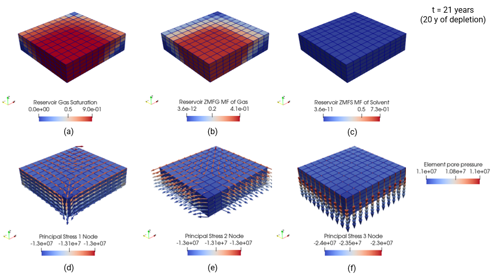
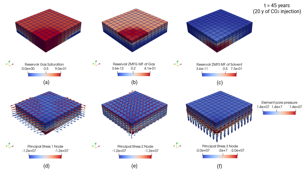
The next two figures below show contour plots for gas saturation, methane gas mass fraction, CO2 solvent mass fraction and pore pressure with principal stress directions and magnitudes indicated by the coloured arrows after 20 years of gas depletion and after 20 years of CO2 injection respectively. Note the change in the directions of the most tensile principal stress (principal stress 1) and the intermediate principal stress (principal stress 2) during those operations. The most compressive principal stress (principal stress 3) remains aligned with the vertical axis throughout the simulation.
Contour plots for gas saturation (a), methane gas mass fraction (b) CO2 solvent mass fraction (c) and pore pressure with principal stress directions and magnitudes indicated by the coloured arrows (d, e, f) after 20 years of gas depletion (t =21 years)
Contour plots for gas saturation (a), methane gas mass fraction (b) CO2 solvent mass fraction (c) and pore pressure with principal stress directions and magnitudes indicated by the coloured arrows (d, e, f) after 20 years of CO2 injection (t =45 years)
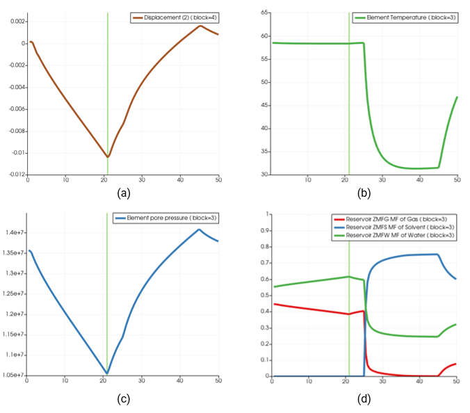
The figure below shows the evolution of different properties obtained from selecting the target cells that will be interrogated and performing a "Plot Selection Over Time" filter. Note how the vertical displacement in the top surface cell above the well (a) is consistent with the evolution of pore pressure in the bottom hole (c). In figure (d) notice how during depletion the gas is slowly being replaced by water in the bottom hole, and then both components are displaced by CO2 at the same location during injection.
Evolution of vertical displacement at top surface in a cell aligned with well location (a). Evolution of element temperature (b), pore pressure (c) and the three components mass fractions (d) in a well cell
|