Ex_003 Transverse Isotropic Elasticity

Contents
In this example a single 3D element is subjected to triaxial test conditions. For simplicity the model geometry has been defined as a cube of 1 m x 1 m x 1 m. The material characterization considers transverse isotropic elasticity with the axis of symmetry being the material axis x3. Note that the convention adopted is that the axes of the material coordinate system will be refereed as x1, x2 and x3 whereas the global coordinate axes will be referred as x, y and z. Several simulations will be performed with different material coordinate system rotations along the x axis. The simulations will consider a confining pressure load on planes perpendicular to x and y axes of 10.3 MPa and a displacement load aligned with the z axis corresponding to 1% of strain. The results from the simulations will be compared to the analytical solution when the axial stress reaches a magnitude of 140 MPa. The transverse isotropic material properties will be:
E11 = 30000 MPa
E33 = 15000 MPa
ν12 = 0.270
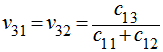
ν31 = 0.225
G13 = 7500 MPa
And from those we can derive:
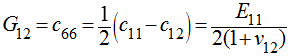
G12 = 11811 MPa
ν23 = 0.450
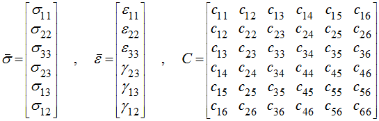
Hooke's law can be expressed in tensorial form as:
where:
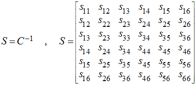
The inverse of the Hooke's law can be expressed as:
where:
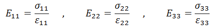
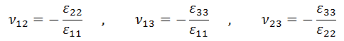
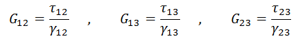
For an orthotropic symmetry the anisotropic elastic properties can be expressed in terms of the Young's modulus, Poisson's ratio and shear modulus on each direction. Those are:
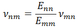
Where
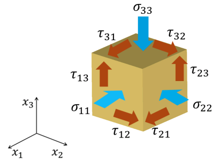
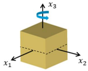
Due to symmetry in stress and strain tensors
Schematic of stresses and strains aligned with the material coordinate system
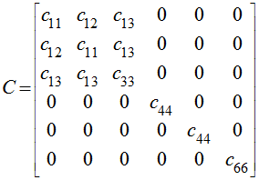
For a transverse isotropic (TI) material in which the axis of symmetry is parallel to axis 3, the stiffness matrix can be written as:
where there are five independent parameters
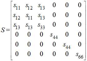
The compliance matrix (
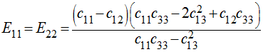
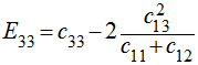
For TI materials the equivalence between the stiffness parameters and the engineering constants is as follows:
And the equivalence between the compliance parameters and engineering constants is as follows:
|


Material coordinate system
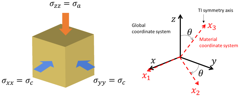
Schematic of problem boundary conditions
This example aims to be a reference for:
•Setting transverse isotropic elastic materials
•Assign rotations to the material coordinate system
The data files for the examples is found in: ParaGeo Examples\General Examples\Ex_003\Data
Note that the data files will be named according to the following convention: Ex_003a_15deg.dat where the last two digits before the file extension indicate the material system rotation along the x axis in degrees.
Material_data
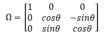
Rotation on material system
|
Results
The result files for the project are in directory: ParaGeo Examples\General Examples\Ex_003\Results.
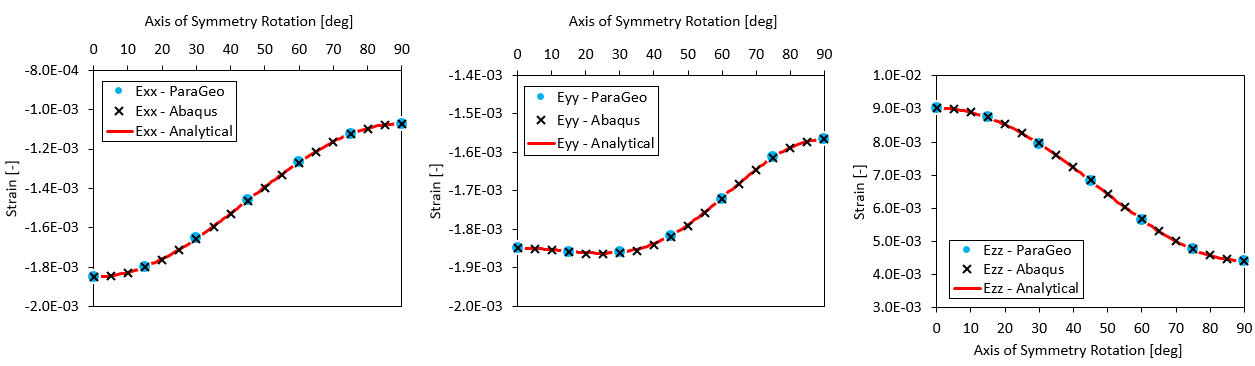
It can be seen that the simulation results match very well the analytical solution for the three strains for different amount of rotations.
Comparison of ParaGeo and Abaqus simulation results for strains in X, Y and Z directions with the corresponding analytical solutions
|