Case02 Facies Mixture-based Material Database

The parameters for defining the yield and flow surfaces shapes for pure lithofacies are defined according the following assumptions:

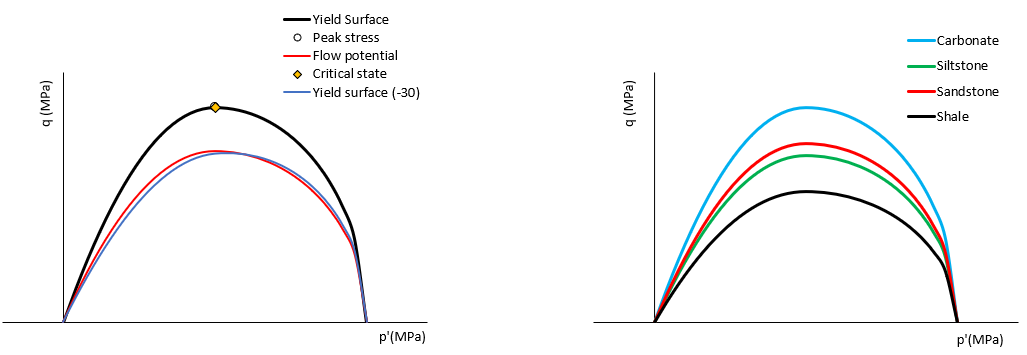
1.Typical values for clays/shales and sandstones are taken into account

2.FA Shale < FA Siltstone < FA Sandstone < FA Carbonates

3.Critical state is located on the peak q point of the yield surface (the yield and flow potential exponents are equal). The assumed value is n = m = 1.

4.Flow potential is defined to be approximately consistent with the yield surface in Reduced Triaxial Extension Tests (RTE) conditions (see in the figure below Yield Surface (-30) )

5.Parameters defining the shape of the yield surface in the deviatoric plane are identical for all lithologies and hence won't be discussed here (α=0.25, β0=0.6, β1=0.6).

Below there are two figures. The one on the left shows the yield surface in both, compression and extension, as well as the flow potential surface for a given lithology. The figure on the right shows the comparison of the yield surfaces for the different pure lithofacies at the same pc and pt values and therefore provides a visual representation of their relative strength. The assumed friction angles for the pure Sandstone, Siltstone, Shale and Carbonate are 32º, 30º, 24º and 38º respectively.

Yield surface in compression, yield surface in extension and flow potential surface shapes for a given material (left). Comparison of yield surfaces at the same pc and pt for the different pure litofacies (right)

The compaction curves are defined using a modified version of the Schneider model but formulated with depth. The equation is very similar to Athy's porosity-depth compaction trend but introduces a minimum porosity, and uses two compressibilities and decomposes the depositional porosity in two fractions as follows:

    with      

Where Ømin is the minimum porosity (assumed 0.01 for all lithologies), Øa and Øb are the two fractions of the depositional porosity Ø0 and ka and kb are the two corresponding compressibilities. With the decomposition of the depositional porosity in two fractions and having separate compressibilities for each fraction this model adds further flexibility relative to Athy's model in defining different compacting curve shapes. Nonetheless for the development of the present database it is assumed that:

    and    

Where k is equivalent to Athy's compressibility.

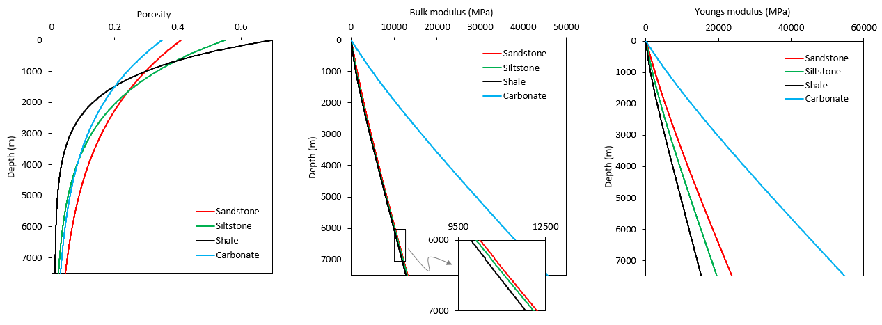
The parameters defining the compaction curves for pure lithologies were obtained from Hantschel and Kauerauf (2009) values for Athy's depth compaction model. In the figure below there is a comparison of those compaction curves (left figure).

Poisson's ratio for pure lithologies was averages from collected values in the bibliography and those were 0.2, 0.25, 0.3 and 0.3 for Sandstone, Siltstone, Shale and Carbonate lithologies respectively. Regarding the poro-elastic parameters it is assumed that the reference bulk modulus is K0=100 MPa and the Aun factor is Aun=0 for all lithologies (appropriate values for geological time scale simulations). The value of κ is defined per lithology according to Young's modulus data collected and has been 0.007, 0.0075, 0.008 and 0.002 for Sandstone, Siltstone, Shale and Carbonate lithologies respectively. In the figure below it is shown the effect of the poro-elastic parameters and Poisson's ratio on Bulk modulus and Young's as a function of depth (centre and right figures).

Compaction curves and corresponding Bulk and Young modulus as a function of depth for pure litofacies

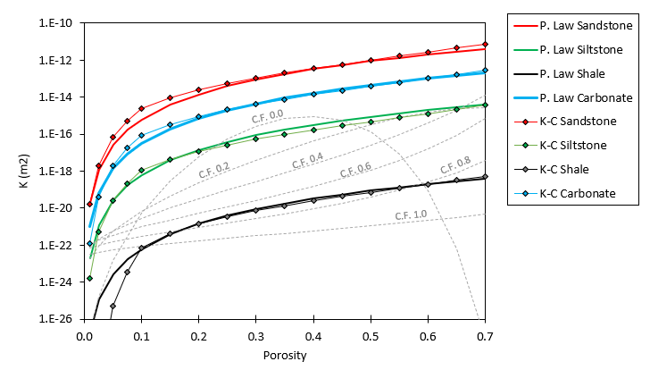
Porosity-permeability curves for each lithology are proposed. Those are modelled using a power law function of the form k=A· Øn with the parameters being calibrated according to Kozeny-Carmen curves provided in Hantschel and Kauerauf (2009). The calibrated power law curves are plotted below compared to the corresponding Kozeny-Carmen curves. A transverse anisotropy factor for each lithology is proposed in the spreadsheet.

Regarding the thermal properties, values for vertical and horizontal grain conductivities as well as the heat capacity are also obtained from Hantschel and Kauerauf (2009).

Comparison of porosity-perm curves for the pure lithofacies. Power law and kozeny-Carmen functions are provided. The grey curves in the background are Yang and Aplin (2010) curves as a function of Clay fraction plotted for reference.

From now onwards the facies will be named according to their component percentages following Ss_Si_Sh_Ca format were SS is percentage of sandstone, Si is percentage of Siltstone, Sh is percentage of Shale and Ca is percentage of carbonate. So for example a lithofacies named 00_15_25_60 is a facies composed of 15 % Siltstone, 25 % Shale and 60 % Carbonate.  

You can find the provided spreadsheet 00_Material_Master_Ss_Si_Sh_Ca.xlsx in Mat_001c/Case02 . This file has 6 sheets in it:

▪Compaction Model Mixtures: This sheet contains the master properties for the pure/single component  lithofacies (cells G4 to AI7) as well as the list of facies with different component mixtures and their corresponding properties calculated from the master ones using percentage-based weighted averages (cells G8 to AI__).

▪Consolidation: Sheet where the hardening table data is calculated (requires some inputs).

▪Permeability: Sheet where the proposed porosity-permeability curve is calculated. Plot of such curve compared to the pure/single component lithofacies curves is provided. (sheet automatically updated)

▪Yield surface: Sheet that provides a plot for the yield surface for the lithofacies being calibrated (sheet automatically updated).

▪k0 test: Sheet to paste history data from a single element oedometer test in order to refine the values for k0 and pc/p' to be input in the "Consolidation" sheet and obtain more accurate hardening values

▪Material_data: Sheet where you can copy paste the whole material being characterised into a .mat file. Orange cells in this sheet are automatically updated for the considered lithofacies, whereas blue cells are fixed values (not recommended to be changed except the characteristic length in regularisation, that may require to be updated in the .mat file according to the application)

The step by step procedure on how to use the material database spreadsheet is as follows:

1.Make a copy of the 00_Material_Master_Ss_Si_Sh_Ca.xlsx file and rename it as Mech_Ss_Si_Sh_Ca.xlsx where Ss_Si_Sh_Ca are the actual percentages of the facies to be characterised (e.g. Mech_00_15_25_60.xlsx). It is proposed to preserve the file named 00_Material_Master_Ss_Si_Sh_Ca.xlsx as a control sheet of the previously validated materials and as a template file to make new copies for new material characterisations.

2.In the "Compaction Model Mixtures" sheet, cell C2, enter the name of the litofacies (e.g. 00_15_25_60) to check whether has been previously characterised. Then there are three possible scenarios:

i.The chosen lithofacies has been previously validated. Then cell D2 will show the facies number in the list (displayed in column I of the table) and cell E2 will show "Validated". Then you should already have the Material_data in a material (.mat) file.

ii.The chosen lithofacies is already defined on the list but has not been validated. Then cell D2 will display the facies number (displayed in column I) and cell E2 will display "None". Then we can jump to step 3 in this step by step guide.

iii.The chosen lithofacies is not defined in the list. Then "Not in the list" is shown in both D2 and E2 cells. Then we need to add it by:

a.Defining its name (following the same SS_Si_Sh_Ca format) in column H after the last row in the table

b.Defining the component percentages in columns J, K, L and M. Values in columns N to AH should automatically be added/updated. Note that the calculated value in column N should be 100 (sum of component percentages).

c.Copy/drag the formula in column I so that a number is assigned to the facies (used for lookup purposes)

3.Jump to "Consolidation" sheet. The name of the target facies to be validated should appear in cell E7. The sheet should automatically display updated properties (Schneider parameters, the orange cells in the table in column C as well as the parameters in the column F).

4.Input the initial guesses for k0 and pc/p' in cells C21 and C22 respectively as well as the remaining missing values in the blue cells from column C. Note that if you hover your cursor above the cells a note with recommended values will be displayed.

5.Jump to "Material_data" sheet and copy-paste the whole data within the thick border (from cell B10 to cell L101) into your material (.mat) file. Note that the properties (including the material name) should automatically be updated for the facies being calibrated.

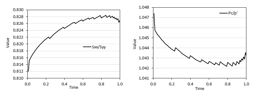
6.Run the Mat_001c_Case01b_k0_test.dat simulation for the defined material. This is a single element oedometer test. Paste the history point results (including headers with the variable names) in the cell AA33 from the "ko test" sheet. From the plots we can derive more accurate values for k0 (Sxx/Syy) and pc/p' than the initial guess values.

Graphs from history results. From these graphs we may assume a stress ratio of 0.828 and a pre-consolidation to effective mean stress ratio of 1.042 to update the spreadsheet input.

7.Replace k0 and pc/p' values in the "Consolidation" sheet, cells C21 and C22 respectively. This will update the hardening table values.

8.Go to "Material_data" sheet and copy again the whole data with the updated/refined hardening values to paste it and overwrite the characterisation in your material (.mat) file.

9.Validate the material characterisation by running a drained consolidation model. This is provided in the datafile Mat_001c_Case01b_cons.dat where gravity is slowly applied to a sediment column and is allowed to compact. Open the results corresponding to the last plot file in ParaView and perform a Plot Over Line in the centre of the column. Export the results in CSV format and copy/paste them (including the headers with variable names) in the cell CH1 from "Consolidation" sheet. Now you can visualize your predicted porosity curve compared to the target curve in the graph located at cell B26 in the "Consolidation" sheet.

10.Add the currently validated facies/material to the list in the master/template sheet file (00_Material_Master_Ss_Si_Sh_Ca.xlsx) and write "Validated" in the cell at G column. This will help to keep track of the previously characterised and validated materials as it will appear on the next copy of the file that you will make to perform an extra material characterisation.

Notes

•It is recommended NOT to modify the 00_Material_Master_Ss_Si_Sh_Ca.xlsx besides adding new facies mixtures to the list and tagged the "Validated" mixtures to keep control of the previously characterised facies mixtures.

•In the Ss_Si_Sh_Ca.mat file material data for the mixtures tagged as "Validated" in the master excel file are provided. Note that some materials have the porosity-permeability curves defined via Kozeny-Carmen model rather than power law (those were created with a previous version of the spreadsheet).

•A copy of the 00_Material_Master_Ss_Si_Sh_Ca.xlsx may be used to create a Master sheet specific to a project (e.g. a given project may require material calibrations for a water density that is different to 1000 kg/m3 which has an impact on the hardening table values, or different master properties for the pure/single component lithofacies may be desired for a project, etc.)

•If different properties than the suggested default ones in this data base need to be considered for a specific facies mixture (e.g. different normal compaction trend, different porosity/perm law) then the properties may be changed manually in the corresponding sheets for that specific material (Mech_Ss_Si_Sh_Ca.xlsx), e.g.:

▪To use a different normal compaction trend than the default one you can manually overwrite the values in cells C7 to C12 from "Consolidation" sheet and repeat the step by step validation procedure described above

▪To use a different power law porosity-perm curve you can manually overwrite values in cells O4 to O6 from "Permeability" sheet. This does not has any effect on the hardening so there is no need to repeat the validation procedure.

▪To use different yield/flow potential surface parameters you can change cells F19 and F20 and repeat the step by step validation procedure described above (note this will have an impact on the k0 (Sxx/Syy) and pc/p'  values.

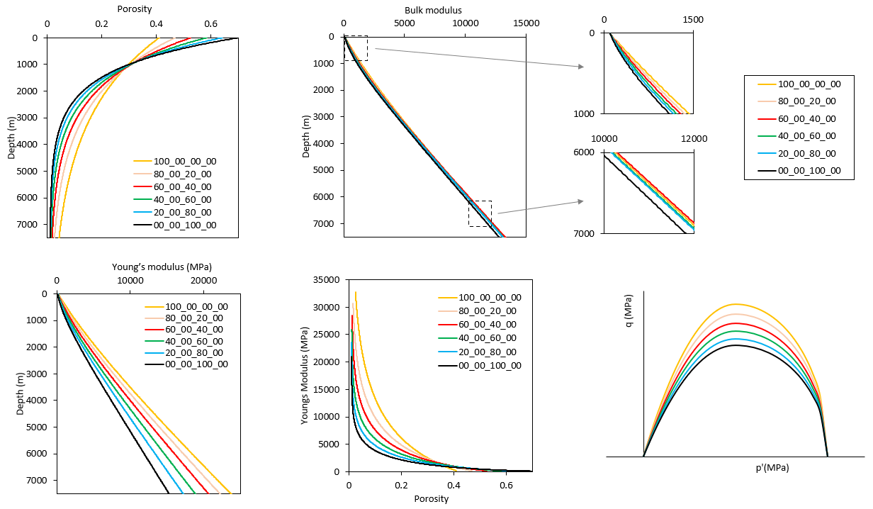
View of some mechanical properties extracted from the data base for different mixtures from pure Sandstone to pure Shale

Hantschel T. & Kauerauf, A. (2009) Fundamentals of Basin and Petroleum Systems Modeling. Springer-Verlag. Berlin Heidelberg 2009.

Yang, Y. & Aplin, A.C. (2010) A permeability-porosity relationship for mudstones. Marine and Petroleum Geology 27 (8), 1692-1697.