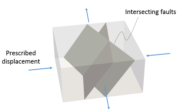
In this example a box shaped domain which contains two intersecting faults is initialized in several stages. The model considers elastic material the 4 initialization stages comprise:
1.Gravity load (with elastic contact)
2.Tectonic displacement on side boundaries (with elastic contact)
3.Contact release
4.Displacement reinitialization

Schematic of problem boundary conditions
This example aims to be a reference for setting mechanical contact data. Several cases will be demonstrated comprising:
•Constant contact stiffness (Ex_001a)
•Field dependent stiffness (Ex_001b)
•Depth dependent stiffness (Ex_001c)
•Stiffness dependent on underlying element stiffness (Ex_001d)
The data files for the examples is found in: ParaGeo Examples\General Examples\Ex_001\Data
Contact Global Data (all examples)
Data File
|
|
* Contact_global
Included_contact_sets IDM=1
"All"
Corrective_step_flag 0
Factor_contact_time_step 0.750000
|
1.Contact_global data is compulsory if contact is active. The active contact sets for the are specified. 2.Initial penetrations will not be corrected (Corrective_step_flag = 0). The corrective step flag is useful when initial contact penetrations in the geometry exist (e.g. when the geometry is derived from a restoration). 3.The Factor_contact_time_step is set to 0.75 so the contact critical time step will be multiplied by 0.75. The time step used to perform the simulation will be the minimum between the contact time step and the element time step.
|
Contact Set Data (all examples)
Data File
|
|
* Contact_set NUM=1
Name "All"
Contact_surfaces IDM=4
"Fault1_ftw"
"Fault1_hgw"
"Fault2_ftw"
"Fault2_hgw"
Global_update_frequency 1000
Buffer_factor 2.0
Field_factor 0.2
Property_name "Fault"
Print_search 1
Contactor_corner_model 0
|
1.In Contact_set data the geometry sets which are considered for contact should be specified. Note that contact surfaces must be previously defined as geometry sets. 2.The Global_update_frequency is set to 1000 steps. This means that every 1000 mechanical steps the contact list with potential target facets is updated. High values can be set if contact nodes are not expected to move distances which are long relative to the element length. 3.Buffer_factor is set to 2. This means that on every update on the contact list, for each contact node the facets within the contact zone (potential target facets) will be those which are at a distance less or equal to dbuff calculated as: dbuff = lcont · fbuff = lcont · 2
where lcont is the side of the facets adjacent to the contact node and fbuff is the buffer factor.
4.Field_factor is set to 0.2. This means that the field distance dfield (distance/penetration over which contact is considered) will be calculated as: dfield = ltarg · ffield = ltarg · 0.2
where ltarg is the target facet length and ffield is the field factor.
5.Contact property named "Fault" is assigned by default to all contact surfaces included in the contact set. 6.Print_search is set to 1 so contact search information will be written in the .res file. 7.Contactor_corner_model is set to 0.
|
Contact Surface Data (all examples)
Data File
|
|
* Contact_surface NUM=1
Name "Fault1_ftw"
Property_name "Fault"
Surface_interaction IDM=1
"Fault1_hgw"
Set_name "All"
* Contact_surface NUM=2
Name "Fault1_hgw"
Property_name "Fault"
Surface_interaction IDM=1
"Fault1_ftw"
Set_name "All"
* Contact_surface NUM=3
Name "Fault2_ftw"
Property_name "Fault"
Surface_interaction IDM=1
"Fault2_hgw"
Set_name "All"
* Contact_surface NUM=4
Name "Fault2_hgw"
Property_name "Fault"
Surface_interaction IDM=1
"Fault2_ftw"
Set_name "All"
|
1. A Contact_surface data structure is defined for each contact surface in the contact set. In such data structure the potential contact interactions for each contact surface are defined. In this case each fault hanging wall can only interact with its corresponding foot wall and vice versa. 2. Specific contact properties may be assigned to different contact surfaces (e.g. Fault 2 may have different contact property than Fault 1). In this case all faults have assigned contact property named "Fault".
|
Data File
|
|
* Contact_property NUM=1
Name "Fault"
Compression_model 1
Compression_properties IDM=1
10000.00
Tangential_model 2
Tangential_properties IDM=2
10000.00 0.6
|
1.The Contact_property is named "Fault". 2.Compression_model is set to 1 (linear elastic model). 3.A contact normal stiffness of 10 GPa is defined 4.Tangential_model is set to 2 (Coulomb model). Thus slip will occur if the tangential force Ft satisfies: Ft > µ · Fn
where µ is the friction coefficient and Fn is the contact normal force.
5.The tangential penalty stiffness is set to 10 GPa and the friction coefficient to 0.6.
|
Data File
|
|
* Contact_property NUM=1
Name "Fault"
Compression_model 1
Compression_properties IDM=1
10000.00
Tangential_model 2
Tangential_properties IDM=2
10000.00 0.6
Field_dep_stiffness_model 1
Field_dep_stiffness_properties IDM=5
0.1 2.0 0.0 0.4 1.002
|
1.The Contact_property is named "Fault". 2.Compression_model is set to 1 (linear elastic model). 3.A contact normal stiffness of 10 GPa is defined 4.Tangential_model is set to 2 (Coulomb model). Thus slip will occur if the tangential force Ft satisfies: Ft > µ · Fn
where µ is the friction coefficient and Fn is the contact normal force.
5.The tangential penalty stiffness is set to 10 GPa and the friction coefficient to 0.6. 6.The Field_dep_stiffness_model is set to 1 so that both the contact normal stiffness and the contact tangential stiffness will be dependent on the penetration. The higher the penetration the higher the stiffness. This is advantageous so that a relatively small stiffness can be used when penetration is small. This can help to prevent high stiffness at zones subjected to low stresses which potentially may be zones of poorly consolidated sediments in evolutionary models at geological time-scale for example, what could result in too big bouncing of the sediment. In addition this can help to increase the size of the contact critical time step as high stiffness will be used only if needed (when penetration is important according to the imposed criteria). 7.Five parameters are required to define the model: i.Lower stiffness factor(Fstifflo): scaling factor for the penalty stiffness at lower reference penetration distance dplo = dfield · Fpenlo, where dfield is the field distance and Fpenlo is the lower penetration factor. ii.Upper stiffness factor (Fstiffup): scaling factor for the penalty stiffness at upper reference penetration distance dpup = dfield · Fpenup, where dfield is the field distance and Fpenup is the upper penetration factor. iii.Lower penetration factor (Fpenlo): multiplication factor for the field distance to calculate the lower reference penetration distance dplo (which is associated to the Lower stiffness). iv.Upper penetration factor (Fpenup): multiplication factor for the field distance to calculate the upper reference penetration distance dpup (which is associated to the Upper stiffness). v.Maximum Change Factor: Maximum change factor in stiffness between consecutive time steps. This is used to prevent sudden stiffness changes which can lead to numerical instabilities. 8.In the present case the considered stiffness for each of the examples penetration distances will be as described in the following table:
Penetration
|
Stiffness
|
0.0 · dfield
|
1000 MPa
|
0.1 · dfield
|
5750 MPa
|
0.3 · dfield
|
15250 MPa
|
0.4 · dfield
|
20000 MPa
|
0.5 · dfield
|
20000 MPa
|
|
Data File
|
|
* Contact_property NUM=1
Name "Fault"
Compression_model 1
Compression_properties IDM=1
10000.0
Tangential_model 2
Tangential_properties IDM=2
10000.0 0.6
Compression_dependent_variables IDM=1
"Depth"
Compression_property_table IDM=4 JDM=2
0.0 500.0 1000.0 2000.0
500.0 5000.0 7500.0 10000.0
Tangential_dependent_variables IDM=1
"Depth"
Tangential_property_table IDM=4 JDM=3
0.0 500.0 1000.0 2000.0
500.0 5000.0 7500.0 10000.0
0.6 0.6 0.6 0.6
|
1.The Contact_property is named "Fault". 2.Compression_model is set to 1 (linear elastic model). 3.A contact normal stiffness of 10 GPa is defined 4.Tangential_model is set to 2 (Coulomb model). Thus slip will occur if the tangential force Ft satisfies: Ft > µ · Fn
where µ is the friction coefficient and Fn is the contact normal force.
5.The tangential penalty stiffness is set to 10 GPa and the friction coefficient to 0.6. 6.Both compression and tangential models are defined to have properties varying with depth. The data is self explanatory. 7.Note that when using depth dependent properties stratigraphy must be defined. |
Data File
|
|
* Contact_property NUM=1
Name "Fault"
Compression_model 1
Compression_properties IDM=1
0.0
Tangential_model 2
Tangential_properties IDM=2
0.0 0.6
Normal_element_stiff_fact 1.0
Tangential_element_stiff_fact 1.0
|
1.The Contact_property is named "Fault". 2.Compression_model is set to 1 (linear elastic model). 3.Tangential_model is set to 2 (Coulomb model). 4.Normal and tangential stiffness specified in contact property will not be used. However they must be specified. 5.Normal_element_stiff_fact and Tangential_element_stiff_fact are used to define a multiplication factor of the group stiffness in order to calculate the normal and tangential contact stiffness respectively. |
|
The result files for the project are in directory: ParaGeo Examples\General Examples\Ex_001\Results.
Note that results for cases Ex_001a (constant stiffness) and Ex_001d (constant stiffness dependent on background element) results are identical as the contact stiffness is the same for both cases. Therefore only results for case Ex_001a are plotted.
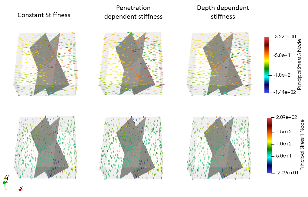
For the three cases (Ex_001a, Ex_001b and Ex_001c) the stresses in X, Y and Z directions are very similar. Direction of principal stresses is also similar.
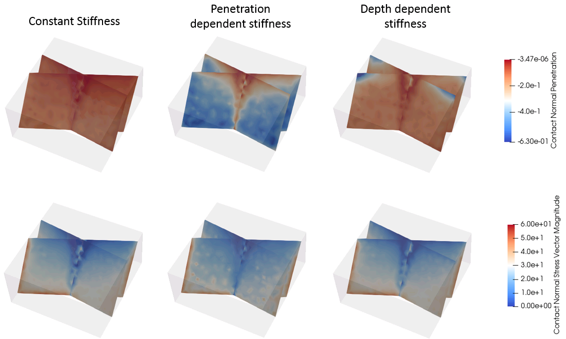
Contact normal penetration is higher for cases with non-constant stiffness, but the value is rather small (0.6 m for a model length of 4000 m). The contact stress vector magnitudes is similar for all cases.
Even though the results are similar with the 3 types of contact properties the CPU times varied significantly. The CPU times normalized relative to the CPU time obtained from case with constant stiffness were:
Ex_001a (constant stiffness) : 100 %
Ex_001b (penetration dependent stiffness) : 43.7 %
Ex_001c (depth dependent stiffness) : 81.9 %
Thus this example shows that in addition to the advantage of avoiding potential problems when using high contact stiffness near surface for weak plastic materials, non-constant stiffness models may help so save CPU time.

Stresses for the three cases

Directions and magnitudes of maximum (top) and minimum (bottom) principal stresses. Note that vector lengths are constant (not scaled).

Contact normal penetration and normal stress magnitude for the three types of contact properties
|
