HM_005 Uniaxial Sedimentation followed by Tectonic Compression

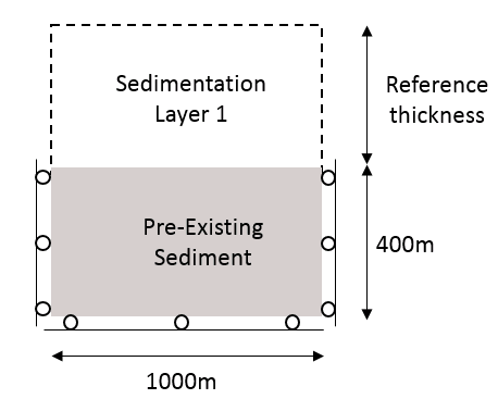
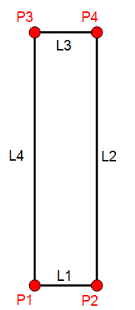
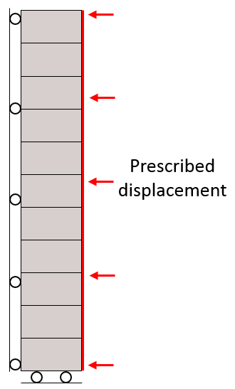
The objective is to simulate the sedimentation and consolidation of 4000m of sediment over a period of 40.0 Ma (sedimentation rate of 100m/Ma) followed by a tectonic compression that will cause 8% of shortening in 0.5 Ma.  The pre-existing sediment height is initially 400 m and consolidates during gravity loading. The width is fixed at 1000 m in order to facilitate the visualization in Paraview. Sedimentation is represented by the "drape" layer sedimentation algorithm. During the sedimentation stage, 10 clay layers with a thickness of 400 m are deposited.

During the sedimentation stage the model is analysed in uniaxial strain conditions; i.e. the vertical sides of the model are constrained in the horizontal direction, and the base of the model is constrained in the vertical direction. Gravity is the only load type and the top surface of the model is prescribed a small mechanical stress load of 0.2MPa to help with surface stability and a zero pore pressure (pf); i.e. free drainage, resulting in a gradual dissipation of pore pressure in the model.  The gravity load for the pre-existing sediment is applied over 4.0 Ma and then sedimentation of the column takes place between 4.0 and 44.0 Ma.  The mesh is structured with quadrilateral elements  ("QPM4" type). The height of each layer is divided in 10 elements whereas a single element covers the whole width (i.e. approaching a 1D model set up).  Adaptive remeshing is not required for this model and therefore the Error_evaluation_frequency keyword data is set with a large number (i.e. to avoid remeshing).

During the tectonic stage a prescribed displacement corresponding to 8% of shortening is applied on the right hand boundary over 0.5 Ma. The tectonic stage is defined as a separate datafile that uses the Restart_read_data data structure to read the results from the sedimentation stage in order to continue the simulation.

Material Properties

The material corresponds to a generic Clay characterization with Kimmeridge Clay properties as a benchmark. A poro-elastoplastic material constitutive model is used to define the material rheology. The material hardening law is defined according to the Hudec et. al. (2009) compaction trend for Golf of Mexico sediments assuming hydrostatic pressures, a grain density of 2650 Kg/m3 and a water density of 1000 Kg/m3. The porosity-permeability relationship is defined using Yang and Aplin (2010) model for a mudstone with clay fraction of 0.4.

The additional material parameters related to the porous flow field are:

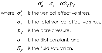
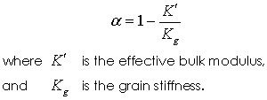
Notes

1The simulation uses a transverse isotropic permeability via definition of Permeability_y_vs_porosity, and Permeability_x_vs_porosity with a horizontal to vertical permeability ratio of 5.0. However the flow is expected to be mainly vertical due to the geometry configuration.

2The Biot constant (Biot_constant) defines the contribution of the pore pressure to the total stress via the effective stress relationship

The Biot constant may either be user defined (as in this case) or may be computed automatically via the relationship

3The material is specified as fully saturated ( Fluid_saturation = 1.0).

4The material is saturated with fluid number 1.

Fluid Properties

The properties of the pore fluid must be specified.  The principal parameters are:

The restart files allow to recover the simulation state at a user specified time and continue the simulation according to the data defined in the Restart data file. This has multiple applications, e.g:

1 Facilitate a parametric study with identical initial stages, so that the initial stage only needs to be run once and the results will be used for all the simulations (e.g. a parametric study of different shortening rates on a column deposited at a defined sedimentation rate)

2 Modify some data at an intermediate time for a given model without the need to run it from the beginning

3 Facilitate the process of overcoming some errors (by saving time) that might be encountered during a simulation (e.g. convergence problems, leaking of material, etc.)

Note that the restart files are created according to the commands specified in the control data (See Basic Set Up: Sedimentation Data File Description).