Case02 With Contact Advection along Fault


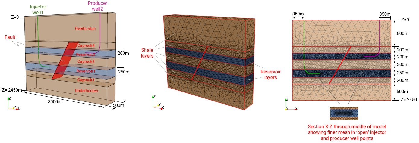
The primary goal of this example is to demonstrate contact advection along the fault.  The cold injection fluid is drawn from the lower reservoir1 up and along the fault to the upper reservoir2.  The example also include definition of well history data.


The files for the project are in directory: ParaGeo Examples\General Examples\Ex_008\Case02. Only the key data associated with usage of well elements, contact property and transient time step growth solution data will be described here. A tutorial on how to generate the geometry for the Case01 example using Gmsh is available in Gmsh_002, albeit with slightly different mesh refinement.  The geometry and mesh for Case02 are similarly created.


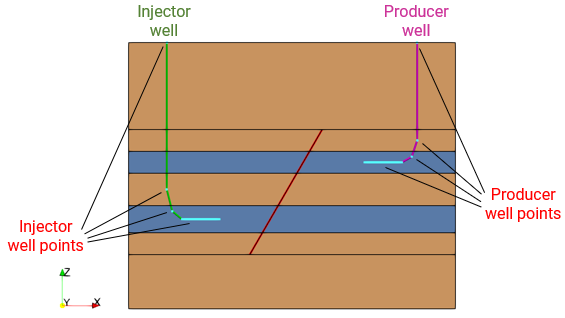
Note that the injection and production wells are not 'active' until stage 4 and 5 respectively, however, it is recommended that the wells are defined in stage 1 with the well points 'shut' and then updated to 'open' when they come online in the later stages.  This enables the user to visualize and track the wells throughout the simulation.


Ex_008b_01


Model and Mesh Definition


Key contact property data with advection (.contact)


Contact advection data is highlighted in bold on the lhs panel below. In this example, the advection conductivity values are defined the same as the layer material grain thermal conductivities.

A one metre damage zone is defined for the fault Contact_width.

Data File


* Contact_property            NUM=1

! ---------------------------------

 Name                       "Fault_sand"    

 Compression_model                     1

 Compression_properties  IDM=1

  /Normal Penalty/           10000.0E6

 Tangential_model                      2

 Tangential_properties   IDM=2              

  /Tangential Penalty/        10000.0E6

  /Friction coefficient/            0.2

 Flow_model_normal                    11

 Flow_properties_normal  IDM=2

  /Intrinsic Perm (Fracture)/      1E-12    

  /Intrinsic Perm (Filter Cake)/   1E-12      

 Flow_model_tangential                11

 Flow_properties_tangential IDM=1

  /Intrinsic Perm/                1E-09  

 Thermal_model_normal                  1 ! 1 - Constant conductivity

 Thermal_properties_normal  IDM=2

  /Therm. Cond. (Penalty)/     3.91E+06 ! (N.m/day)/m/K  4.53E1 W/m/K

  /Therm. Cond. (Filter Cake)/  3.91E+06 ! (N.m/day)/m/K  4.53E1 W/m/K

Thermal_model_tangential              1 ! 1 - Constant conductivity

 Thermal_properties_tangential IDM=1

  /Therm. Cond. (Penalty)/      3.91E+05 ! (N.m/day)/m/K  4.53 W/m/K

 Specific_heat_model                   1 ! 1 - Constant specific heat

 Specific_heat_properties      IDM=2

  /Bulk Specific Heat/            1223 ! J/Kg/K

  /Bulk Density/                   2221 ! Kg/m3

Contact_width                       1.0 ! 1m damage zone


* Contact_property            NUM=2

! ---------------------------------

 Name                       "Fault_shale"    

 Compression_model                     1

 Compression_properties  IDM=1

  /Normal Penalty/           10000.0E6

 Tangential_model                      2

 Tangential_properties   IDM=2              

  /Tangential Penalty/        10000.0E6

  /Friction coefficient/            0.2

 Flow_model_normal                    11

 Flow_properties_normal  IDM=2

  /Intrinsic Perm (Fracture)/      1E-18    

  /Intrinsic Perm (Filter Cake)/   1E-18      

 Flow_model_tangential                11

 Flow_properties_tangential IDM=1

  /Intrinsic Perm/                1E-09  

 Thermal_model_normal                  1 ! 1 - Constant conductivity

 Thermal_properties_normal  IDM=2

  /Therm. Cond. (Penalty)/     2.27E+06 ! (N.m/day)/m/K  2.63E1 W/m/K

  /Therm. Cond. (Filter Cake)/  2.27E+06 ! (N.m/day)/m/K  2.63E1 W/m/K

Thermal_model_tangential              1 ! 1 - Constant conductivity

 Thermal_properties_tangential IDM=1

  /Therm. Cond. (Penalty)/      2.27E+05 ! (N.m/day)/m/K  2.63 W/m/K

 Specific_heat_model                   1 ! 1 - Constant conductivity

 Specific_heat_properties      IDM=2

  /Bulk Specific Heat/            1390 ! J/Kg/K

  /Bulk Density/                   2073 ! Kg/m3

Contact_width                       1.0 ! 1m damage zone


1Contact_property data structure is defined for two fault contact properties, "Fault_sand" and "Fault_shale".  The following describes that for "Fault_sand" :

a.Name - Defines the name of the contact property as "Fault_sand".

b.The following keywords define the geomechanical contact properties:

i.Compression_model = 1 - Defines the contact compression model as linear elastic.

ii.Compression_properties - Defines the normal compression stiffness/penalty as 10000E6 Pa.

iii.Tangential_model = 2 - Assigns the Coulomb friction model to be used for tangential contact.

iv.Tangential_properties - Defines the tangential stiffness/penalty as 10000E6 Pa and the friction coefficient as 0.2.

c.The following keywords define the porous flow contact properties:

i.Flow_model_normal = 11 - A constant intrinsic permeability model is defined to be used for the contact normal flow.

ii.Flow_properties_normal - The intrinsic perm for flow normal to the contact for both the fracture and filter cake is defined as 1E-12 m2.

iii.Flow_model_tangential - A constant intrinsic permeability model is defined to be used for the contact tangential flow.

iv.Flow_properties_tangential - The intrinsic perm for the tangential flow in the fracture is defined as 1E-9 m2.

d.The following keywords define the thermal heat transfer contact properties*.  Contact advection keyword data are highlighted in bold on the lhs panel:

i.Thermal_model_normal = 1 - A constant thermal conductivity model is defined to be used for the contact normal heat transfer.

ii.Thermal_properties_normal - The thermal conductivity for heat transfer normal to the contact for both the fracture and filter cake is defined as 3.91E6 (N.m/day)/m/K.  Note that this is equivalent to 45.3 W/m/K but scaled to the model time units of "days".

iii.Thermal_model_tangential - A constant thermal conductivity model is defined to be used for the contact tangential heat transfer/advection.

iv.Thermal_properties_tangential - The thermal conductivity for advection along the fault is defined as 3.91E5 (N.m/day)/m/K.  Note that this is equivalent to 4.53 W/m/K but scaled to the model time units of "days".

v.Specific_heat_model - A constant specific heat model is defined to be used for the specific heat for contact advection.

vi.Specific_heat_properties - The bulk specific heat for advection along the fault is defined as 1223 J/kg/K and the bulk density as 2221 kg/m3.

e.Contact_width - The damage zone is set as 1m.


2"Fault_shale" contact property #2 is similarly defined as for "Fault_sand" contact property #1 but with different property values.


*Note that in this THM coupled example, the model time unit is defined as "days" and the thermal scaling option chosen is to manually scale the thermal conductivity values for the time unit, i.e. (N.m/day)/m/K and as such, the specific heat value can be defined in J/kg/K units.  Other alternative thermal scaling options are described in Ex_007 Case01.


Key data for well definition in Stage 1 with well history


Well_definition #1 (Injection well)

Data File


* Well_definition            NUM=1

! ---------------------------------

 Name             "Inj_well1"

 Well_path         IDM=3  JDM=27 ! Need to define top to bottom for well elements  

    350  250   0

    350  250  -1350

    400  250  -1550

    490  250  -1625

    505  250  -1625

    520  250  -1625

    ....           ! Horizontal section of well points every 15m

    820  250  -1625

    835  250  -1625

 Well_radius           1.00

 Status_distribution   IDM=27

   "casing"

   "shut"

   "shut"

   "shut"

   "shut"

   "shut"

    ....

   "shut"

   "shut"

 Injection_rate           5000   ! m^3/day

 Well_temperature         30.0

 Time_curve               200

 Singlephase_fluid_name  "Water"

 Flow_model               3     ! Hydrostatic prescribed well

 Output_level             1

History_summ_frequency   1     ! Use default name and output every step


* Time_curve_data          NUM=200

! --------------------------------------

 Name                    "Injection"  

 Time_curve    IDM=2

   3.0   13.0

 Load_factor   IDM=2

   0.0   1.0


1Well_definition data structure is defined for the injection well #1:

a.Name - The injection well is named "Inj_well1".

b.Well_path - Defines the x, y and z coordinates of the 27 well points from top to bottom.

c.Well_radius - A constant well radius of 1.0 m is defined.

d.Status_distribution - The status distribution for all well points is defined as "casing" (no leak off) at the top and "shut" (no leak off) for all other well points at the start of the simulation.  Note that the "shut" status will be changed to "open" in the horizontal section of the well during the injection stage.

e.Injection_rate - An injection rate of 5000 m3/day is defined and applied via the Time_curve 200.

f.Well_temperature - A constant injected well fluid temperature of 30 °C is defined.

g.Singlephase_fluid_name - The well fluid is defined as "Water", same as the pore fluid in the formation.

h.Flow_model - The well flow model is defined as hydrostatic prescribed based on surface pressure (default).

i.Output_level - The level of output detail of well information (pressure/flow rates) in the .res file is defined as 1 (standard).

j.History_summ_frequency set to 1 defines the output of well history data every step using the well name as default.


2Time_curve_data 200 defines the time curve associated with the well loading, in this case, the Injection_rate which is applied as a linear ramp over 10 days.


Ex_008b_02

Injector and Producer well points definition


Well_definition #2 (Production well)

Notice that Well_temperature is not defined for the production well as it only makes sense to define this data for the injected well fluid.


Data File


* Well_definition            NUM=2

! ---------------------------------

 Name             "Prod_well2"

 Well_path         IDM=3  JDM=27 ! Need to define top to bottom for well elements  

    2650  250   0

    2650  250  -900

    2600  250  -1050

    2510  250  -1100

    2495  250  -1100

    2480  250  -1100

    ....           ! Horizontal section of well points every 15m

    2180  250  -1100

    2165  250  -1100

 Well_radius           1.00

 Status_distribution   IDM=27

   "casing"

   "shut"

   "shut"

   "shut"

   "shut"

   "shut"

    ....

   "shut"

   "shut"

 Production_rate          5000   ! m^3/day

 Time_curve               300

 Singlephase_fluid_name  "Water"

 Flow_model               3     ! Hydrostatic prescribed well

 Output_level             1

History_summ_frequency   1     ! Use default name and output every step


* Time_curve_data          NUM=300

! --------------------------------------

 Name                    "Production"  

 Time_curve    IDM=2

   13.0   23.0

 Load_factor   IDM=2

   0.0   1.0


1Well_definition #2 data structure is defined for the production well (see picture above):

a.Name - The production well is named "Prod_well2".

b.Well_path - Defines the x, y and z coordinates of the 27 well points from top to bottom.

c.Well_radius - A constant well radius of 1.0 m is defined.

d.Status_distribution - The status distribution for all well points is defined as "casing" (no leak off) at the top and "shut" (no leak off) for all other well points at the start of the simulation.  Note that the "shut" status will be changed to "open" in the horizontal section of the well during the injection stage.

e.Production_rate - A production rate of 5000 m3/day is defined and applied via the Time_curve 300.

f.Singlephase_fluid_name - The well fluid is defined as "Water", same as the pore fluid in the formation.

g.Flow_model - The well flow model is defined as hydrostatic prescribed based on surface pressure (default).

h.Output_level - The level of output detail of well information (pressure/flow rates) in the .res file is defined as 1 (standard).

i.History_summ_frequency set to 1 defines the output of well history data every step using the well name as default.


2Time_curve_data 300 defines the time curve associated with the well loading, in this case, the Production_rate which is applied as a linear ramp over 10 days.


Key data for well definition in Stage 4 injection and Stage 5 production


Once the wells come online, the well data previously defined in stage 1 still applies and the re-definition well data need only consist of the name of the well, the status distribution (and well loading time curve if different from previously defined).


Well_definition #1 (Injection well)

Data File


* Well_definition            NUM=1

! ---------------------------------

 Name             "Inj_well1"

 Status_distribution   IDM=27

   "casing"

   "shut"

   "shut"

   "open"

   "open"

   "open"

    ....

   "open"

   "open"


1Well_definition #1 data structure is re-defined for the injection well #1 in stage 4 injection:

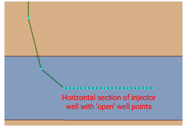
a.Status_distribution - The status distribution for all "shut" well points along the horizontal section of the well in the reservoir layer is changed to "open".

Ex_008_03a

Injector 'open' well points in reservoir layer


Well_definition #2 (Production well)

Data File


* Well_definition            NUM=2

! ---------------------------------

 Name             "Prod_well2"

 Status_distribution   IDM=27

   "casing"

   "shut"

   "shut"

   "open"

   "open"

   "open"

    ....

   "open"

   "open"


1Well_definition #2 data structure is re-defined for the production well #2 in stage 5 production:

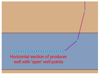
a.Status_distribution - The status distribution for all "shut" well points along the horizontal section of the well in the reservoir layer is changed to "open".

Ex_008_03b

Producer 'open' well points in reservoir layer


Key data for solution control in Stage 6 injection and production flow over pseudo-84 years duration


To demonstrate contact advection up and along the fault to the produced upper reservoir layer, a pseudo long duration of 84 years is simulated. It is not uncommon in reservoir injection and production simulations which take place over a long duration (typically 15 to 30 years) that steady-state flow occurs where the pore pressure in the injected/depleted reservoir remains constant.  Under these conditions, the model simulation does not require small time steps to capture the change in pore pressure as there is little/no pore pressure change, hence the simulation can be performed using large time step increments.  To achieve this, a transient time step growth factor in the solution control data can be defined.


Data File


* Control_data

! ---------------------------------

 Control_title         "Inject Prod Flow"

 Solution_algorithm               4

 Duration                    30660.0 ! 30660 days = 84 years

 Initial_time_increment         0.5

 Maximum_time_increment       200.0

 Transient_time_step_growth    1.04  

 Target_number_time_steps       200

 Output_frequency_plotfile       -1

 Output_time_plotfile        1000.0

 Output_frequency_restart        -1

 Screen_message_frequency        10  


1Three keyword data in the solution Control_data data structure allows for the definition using a transient time step growth for the time increment:

a.Initial_time_increment - this defines the initial time step increment.

b.Maximum_time_increment - this defines the maximum time step increment permitted.

c.Transient_time_step_growth - this defines the factor for which the time step increment will 'grow' from one step to the next.


Note that the final time step increment for the stage will be cut to link up with the stage duration. So, for example, if the termination time is 30683 and a maximum time increment of 200 is achieved at time of 30680, the final time increment will be 3 instead of 200 to achieve the stage termination time.


Results

The result files for the project are in directory: ParaGeo Examples\General Examples\Ex_008\Case02\Results.


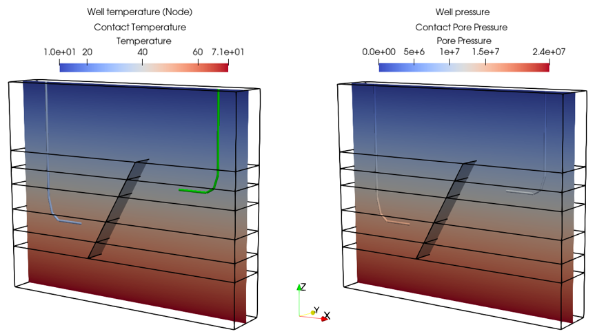
The results below show the initial condition of the model with depth-dependent spatial temperature gradient from 10°C at the surface to 71°C at the base of the model and hydrostatic pore pressure for the whole model.  Injected well temperature is at 30°C.


Ex_008b_03

Initial Condition: Depth-dependent spatial temperature gradient and hydrostatic pore pressure


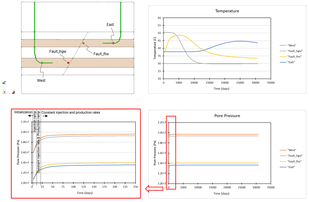
Below shows the plots of temperature and pore pressure distribution throughout the simulation time at four history points located in the injected and depleted reservoir layers.  Notice that the pore pressure is near constant after 230 days with maximum over-pressure of c.a. 3.7MPa in the vicinity of the injected 'open' well point 'west'.  The heat transfer of the well injected temperature of 30°C from 'west' to 'east' progresses slowly through time with the fault hanging wall (grey curve) only 'seeing' the injected fluid temperature after 10,000 days (c.a. 27years).  The fault footwall (gold curve) in the produced upper reservoir layer initially 'sees' an increase in fluid temperature from the higher temperature lower reservoir transported through advection.  This is followed subsequently with a decrease in fluid temperature when the colder injection fluid reaches this history monitoring point.


Ex_008b_04

History points in injected/depleted reservoir layer and the temperature and pore pressure distribution at these points over simulated model time


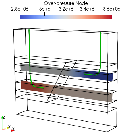
Constant over-pressure in both reservoir layers is observed in the plot below 230 days of injection and depletion with maximum over-pressure of c.a. 3.6MPa in the injected lower reservoir and c.a. 2.8MPa in the produced upper reservoir.


Ex_008b_05

Over-pressure in the two reservoir layers


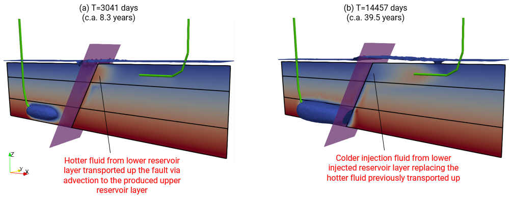
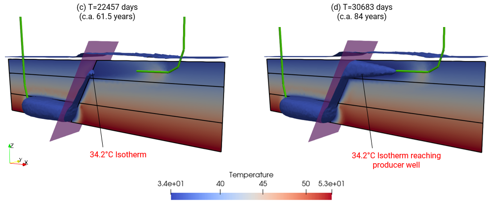
The evolution of the 34.2°C isotherm and temperature distribution from advection (including along the fault) is shown in the plots below in the two reservoir layers with caprock sandwiched in between. Plot (a) shows the hotter fluid from the lower reservoir layer transported up and along the fault to the upper reservoir layer via advection.  In plot (b), this fluid is subsequently replaced by the colder injection fluid along the same flow path up the fault.  Plot (c) shows the progression of the 34.2°C isotherm into the upper reservoir layer and reaching the producer well in plot (d).


Ex_008b_06a


Ex_008b_06b


Evolution of 34.2°C isotherm and temperature distribution showing advection flow along the fault from lower reservoir injector well to upper reservoir producer well