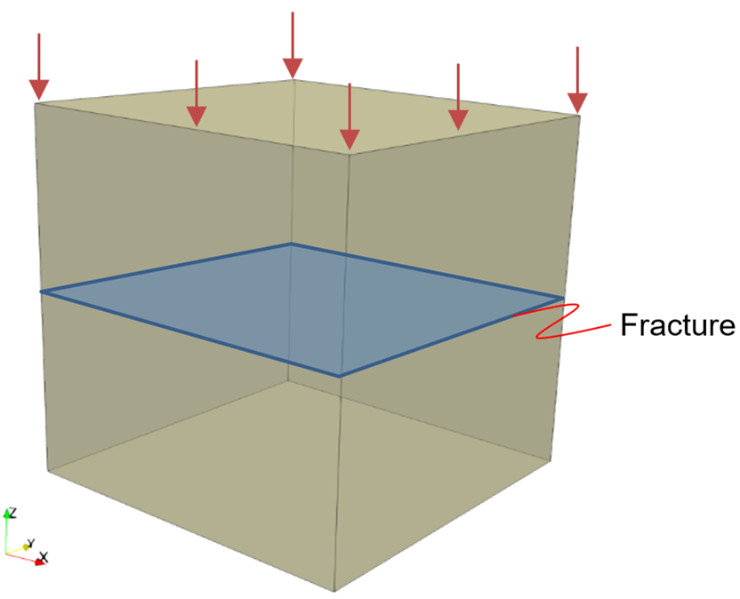
Case03 Joint Normal Displacement with Cyclic Loading

Contents

This example comprises a single hexahedral element (1m x 1m x 1m) subjected to uniaxial displacement. The element contains a single fracture orientated in the horizontal plane with the properties listed below. The fracture spacing corresponds to the height of the element so there is a single fracture in the element. The axial displacement is initially loaded to peak load, then cycled to 50% of the peak load and back to 100%.

Note that the data file for this Case03 example differs from the Case01 data file in just the cyclic loading time curve Time_curve_data data structure and an additional history output for fracture normal stress variable "F_nstrs".

$fract_003_case03_fig1$

Fig. 1 Prescribed loading on element with embedded continuum fracture

Material Properties

The properties used in this simulation are listed below.

Property	Value
Young's Modulus	2000 MPa
Poisson's Ratio	0.20
Porosity	0.35

The additional material parameters related to the embedded fracture are:

Contact Surface Properties	Value
Normal stiffness	1000 MPa
Initial aperture	0.01m
Initial porosity	0.01
Maximum joint stiffness	30000 MPa
Spacing	1.0 m

Data File Description

The data file for the example is in: fract_003\Data\fract_003_case03.dat. The basic data includes:

1Material_data defines the material properties of the model, including the fracture set associated with the embedded fracture.

2Fracture_data assigns the properties of embedded fracture as well as the fracture spacing and local coordinate system.

3Global_loads prescribes axial displacement on the element top surface.

4History_point outputs displacement, stress values, and fracture state variables at every 0.01s.

Note that only key data structures are described below.

Material_data

Material_data defines the material properties of the model, including the fracture set associated with the embedded fracture.

Data File

*Material_data NUM=1

! ---------------------------------

Material_name "Sample"

Units IDM=4

/Stress/ "MPa"

/Length/ "m"

/Time/ "s"

/Temperature/ "Celsius"

Grain_stiffness 3.0000E+10

Grain_density 2710.00

Porosity_model_type 1

Porosity 0.35000

Elastic_model_type 1

Isotropic_elastic_properties IDM=2

/Young's Modulus (E)/ 2000

/Poisson's Ratio (V)/ 0.20000

Fracture_set_names IDM=1

"fract_set1"

1Material name, units and grain stiffness are defined as listed.

2Density is defined as 2710 kg/m3.

3Constant porosity type model is used. The value is defined as 0.35.

4Young’s modulus and Poisson’s ratio are defined as 2000MPa and 0.2, respectively.

5The material data structure is associated with the fracture set “fract_set1”.

Fracture_data

Fracture_data assigns the properties of the embedded fracture as well as the fracture spacing and local coordinate system.

Data File

* Fracture_data NUM=1

! ---------------------------------

Name "fract_set1"

Units IDM=4

/Stress/ "MPa"

/Length/ "m"

/Time/ "s"

/Temperature/ "Celsius"

Propagation_model_name "PreExist"

Fracture_spacing 1.00

Coordinate_system_name "Fracture_Set1"

Normal_stiffness_model "Bandis"

Normal_stiffness_properties IDM=3

/Joint Stiffness/ 1000

/Initial Aperture/ 0.01

/Maximum Joint Stiffness/ 300000

Normal_strength_model "Elastic"

1Fracture data name and units are defined as listed.

2The propagation model type is set as “PreExist”, indicating the embedded fracture as a pre-existing entity.

3Fracture spacing is defined as 1.00m.

4The fracture data is associated with the coordinate system named “Fracture_Set1”.

5The fracture normal stiffness model is defined as Bandis model.

6The input values for Bandis model are defined, including joint stiffness, initial aperture and maximum joint stiffness.

7Elastic normal strength model is defined, indicating no formal failure criterion is applied.

Time_curve_data

Time_curve_data defines the load factor at different times to achieve cyclic loading.

Data File

* Time_curve_data NUM=1

! --------------------------------

Time_curve IDM=4

0.0 0.5 0.75 1.0

Load_factor IDM=4

0.0 1.0 0.50 1.0

1Cyclic loading is defined by setting 100% peak load at t = 0.5s, cycled to 50% of the peak load at t = 0.75s, and back to 100% at t=1s.

Global_loads

Global_loads prescribes axial displacement on the element top surface.

Data File

* Global_loads NUM=1

! --------------------------------

Prescribed_displacement IDM=3 JDM=1

/Set 1/ 0.0 0.0 -0.025

Pres_displacement_geom_set IDM=1

"Top"

Pres_displacement_geom_ass IDM=1

1Geometry set “Top” is prescribed with downward axial displacement of 0.025m.

History_point

History_point outputs displacement, stress values, and fracture state variables at every 0.01s.

Data File

* History_point NUM=1

! --------------------------------

Name "Set1"

Group 1

Output_frequency_time 0.01

Point_coordinates IDM=3 JDM=1

1.0 1.0 1.0

Displacements IDM=1

"DISP_Z"

Stresses IDM=3

"STRS_XX" "STRS_YY" "STRS_ZZ"

Fracture_state_variables NUM=3

"F_kn" "F_dispn" "F_nstrs"

1The History_point data structure is associated with Group 1.

2The history data is output at an interval of 0.01s throughout the simulation time.

3The history data is monitored at coordinate point (1,1,1).

4Displacement, stresses and fracture state variables as listed are output at the monitored history point.

Results

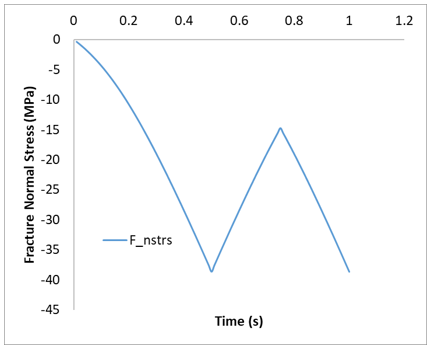
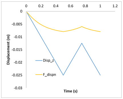
The result files for this example is available in directory: fract_003\Results. In the first compression stage, the results follow the same trend as in Case01, whereby the tangent modulus gradually increases as loading increases. When reaching the peak load at time=0.5s, the load is cycled back to 50% of the peak load and back to 100%.

$fract_003_case03_fig2$

Fig. 2 Axial stress development

$fract_003_case03_fig3$

Fig. 3 Comparison of axial and fracture displacement