Overview

 

ParaGeoInv is a generic tool developed for performing inverse analysis and optimisation of material properties (including geomechanical and porous flow applications) and boundary conditions according to expected known target results. The implemented inversion method is based on the Nearest Neighbour Algorithm, thus allowing inversion of arbitrary sets of parameters from one or several arbitrary experimental / model set-ups. Given a selection of optimisation variables (e.g. permeability and Klinkenberg slippage factor), the algorithm is designed to minimise the misfit value (i.e. difference between the target and model solutions) during the inverse analysis and find the optimal values for the variables. In addition to the default application platform (i.e. ParaGeo), ParaGeoInv can be tailored to work with a variety of simulation tools, such as Eclipse, Abaqus, ELFEN, etc. This flexibility renders ParaGeoInv an analysis-independent tool.

 

This is a useful numerical tool, especially for experimentalists seeking to invert mechanical and/or flow properties of geomaterial under study. In addition to laboratory applications (inversion of material properties), users interested in large-scale geomechanical modelling may benefit from ParaGeoInv, which can conveniently homogenise properties contributed by some geological entities from a much smaller length scale (e.g. fractures) that are populated across the model. Also ParaGeoInv is used for boundary condition optimisation in large scale models as demonstrated in the tutorial example MEM_003.

 

A number ParaGeoInv applications focused on material property inversion are demonstrated in ParaGeoInv Tutorial Examples, but the expectation is that the list will grow as ParaGeo solver is enhanced over time. One example is the characterisation of flow properties in a pulse-decay experiment.

 

 

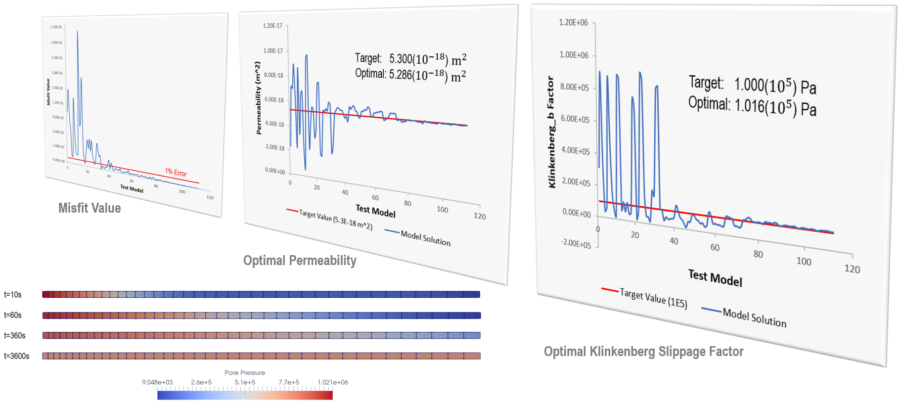
Pulse decay experiments are routinely used to measure petrophysical properties of tight cores by flowing helium. This shows, as part of tutorial example, the finding of optimal permeability and Klinkenberg slippage factor corresponding to core sample, while maintaining low misfit value, i.e. small difference against target solutions which, in this case, are the pore pressure evolution at both inlet and outlet.

 

 

 

ParaGeoInv Workflow

 

The inverse analysis workflow requires the following ingredients:

 

i.Target solution: Defines the target solution that we wish to achieve in a simulation by optimizing the selected parameter(s). This is often a value obtained experimentally. The solutions from the simulations performed during the inversion analysis will be compared to the target solution to evaluate the Misfit (i.e. error relative to the target solution).  

 

ii.Optimization parameter(s) : Parameter(s) being optimized for which the inversion analysis is performed. The optimal value of such parameter should provide an optimal simulation fit to the target solution. An initial range of potential values for such parameter(s) must be defined by the user.

 

iii.Template data file: A ParaGeo data file that defines the geometry, material properties and boundary conditions required to simulate the target experimental setup which provided the target solution. Such template will be used to generate the numerous simulation data files that will be run during the inversion analysis. The template data file must be fully populated with "dummy" values for the inverted / optimized parameters that will be overwritten during the inversion analysis.

 

iv.Inversion analysis data file: File defining the inversion analysis options (e.g. range of potential values for the inverted parameters, Misfit tolerance, number of iterations to be performed, etc). Such file has an .inp extension.

 

The inverse analysis is performed by running the inversion analysis (.inp) data file using the executable ParaGeoInv; e.g. "parageoinv filename.inp". The template data file is used to generate an initial set of "n" simulation data files (here called sample). The number of simulations included in such initial sample is user defined in the inversion analysis data file. Such simulation data files in the sample are copies of the template with the input values of the inverted / optimized parameter(s) being overwritten using random values within the user-defined range. The simulations are run by ParaGeo obtaining a set of "n" solutions.  

 

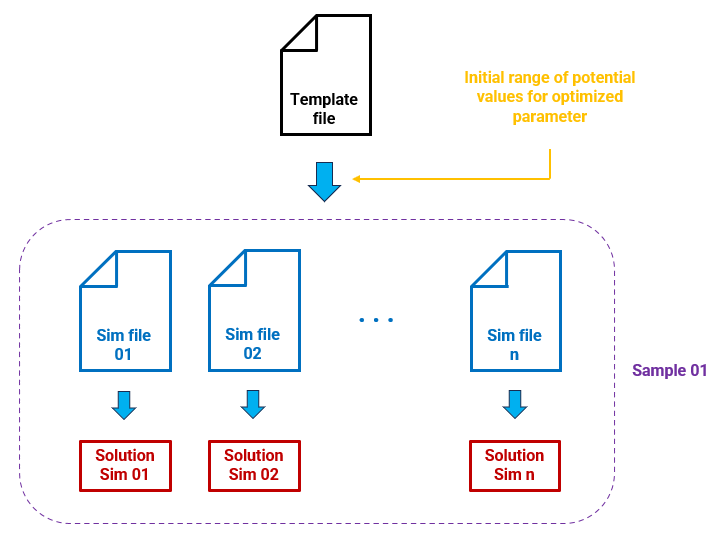
Generation of initial sample of "n" simulations from the template file and the user-defined range of potential values for the parameter being optimized

 

 

 

The solutions of such simulations are evaluated by comparing them to the target solution. The Misfit (error relative to the target solution) for each simulation is calculated and the simulations are ranked from best to worst based on the Misfit information.

 

 

 

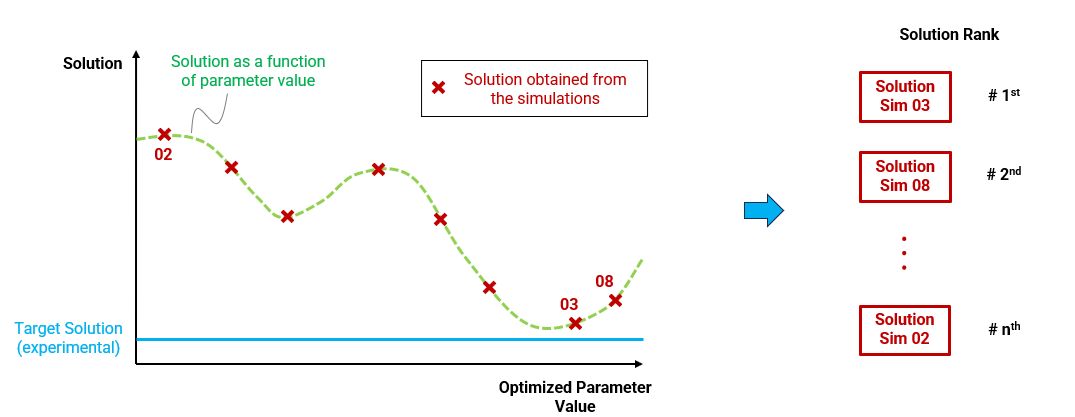
Schematic of the solutions obtained from the initial sample of simulations and their corresponding rank

 

 

 

The best "k" models from the rank (with k being user-defined) are used to establish new maximum and minimum bounds of potential values for the inverted parameter via the nearest neighbour algorithm. Hence the range of potential input values should be narrower relative to the initial/previous iteration.

 

 

 

 

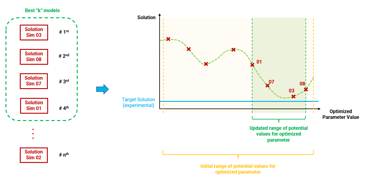
Selection of the best "k" models from the initial solution sample to update the range of potential values for the parameter being optimized

 

 

 

The updated range of potential values for the inverted parameter(s) is used to generate a new sample of "m" simulation data files (re-sample). The number of simulations "m" in re-sample is user-defined. It should be noted that the number of simulation data files in the re-sample should be equal or less than the simulations in the initial sample (m ≤ n).

 

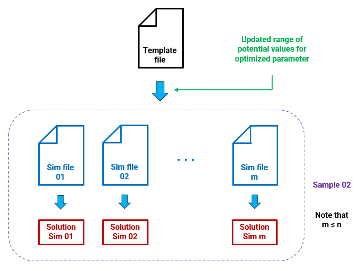
Generation of a re-sample of "m" simulations from the template file and the updated range for the optimized parameter

 

 

The new set of results will be compared again to the target solution and the Misfit will be evaluated. New re-samples (iterations) are performed until either:

 

i.the Misfit value is below a user-defined tolerance and hence we have optimized the value for the inverted parameter

 

ii.the inversion analysis reaches a user-defined maximum number of re-samples (iterations) before the Misfit converges below the tolerance

 

The second case may happen for numerous reasons; e.g.:

 

i.We are trying to invert several parameters at once which may difficult convergence

 

ii.The parameters that we are inverting for may be have a degree of inter-dependence for the modelled scenario and hence there may be different combinations of such values that would decrease the Misfit (i.e. non-unique solution)

 

iii.The inversion analysis may get stuck in a local minima and hence do not converge to an optimal value for the inverted parameter. This may happen for example if the number of simulations considered in each re-sample is too small (this is case dependent)

 

iv.The simulation/system is poorly constrained

 

The general iterative workflow of the inverse analysis using ParaGeoInv is illustrated below.

 

 

 

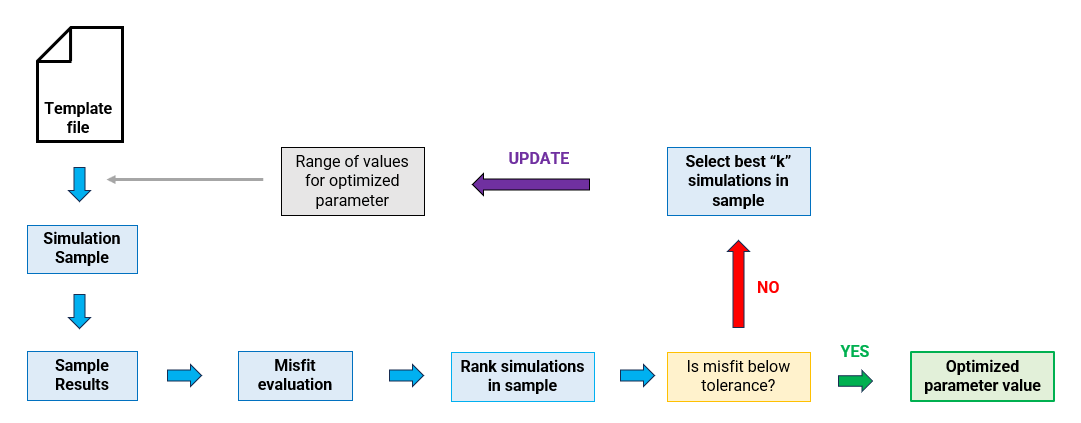
General workflow of ParaGeoInv

 

 

Inverse analysis applications

 

Currently there are two main inversion types / applications supported:

 

•Material:  we invert / optimize any properties and parameters defined within Material_data, Fracture_data, and Fluid_properties data structures (some examples listed below).

 

•Boundary: we aim to optimize the boundary displacement in a model for calibration purposes. It should be noted this is a research-type of application