Introduction

 

This section contains a series of tutorial examples, demonstrating the use of ParaGeoInv in recovering properties that are specified under Material_data, Fracture_data and Fluid_properties data structures. Overview of ParaGeoInv and the inverse analysis and data structures are provided in ParaGeoInv Reference Manual.

 

By the end of this tutorial, the user should be more familiar with:

1.Linking the directories of test, template and target data files in a single ParaGeoInv data file

2.Setting up optimisation parameters (e.g. range of values, corresponding data structure and numbers)

3.Tuning algorithm parameters (e.g. convergence tolerance, maximum number of samples, number of models for (re)sampling, etc.)

4.Specifying misfit data set for comparison between model and target solutions

5.Evaluating the quality of results by the evaluation of misfit value and optimal solutions

 

 

It should be noted that an inverse analysis consists of an iterative process in which numerous simulations are run with the aim to find the optimal model with inverted parameters that allow a good fit with a target solution. Generally the target solution consists of experimental and/or field observations. Nonetheless, for demonstrative purposes the target solutions used in the following tutorial examples are generated from ParaGeo reference simulations which are also provided to the user.

 

Note that the example MEM_003 provided within ParaGeo Tutorial Examples chapter also demonstrates usage of ParaGeoInv for performing an inversion analysis. Such example focuses on boundary displacement optimisation in a large scale model setting rather than inverting for material properties and hence is provided in another section of the manual.

 

 

Tutorial Examples

 

GeoInv_001: Footing settlement

 

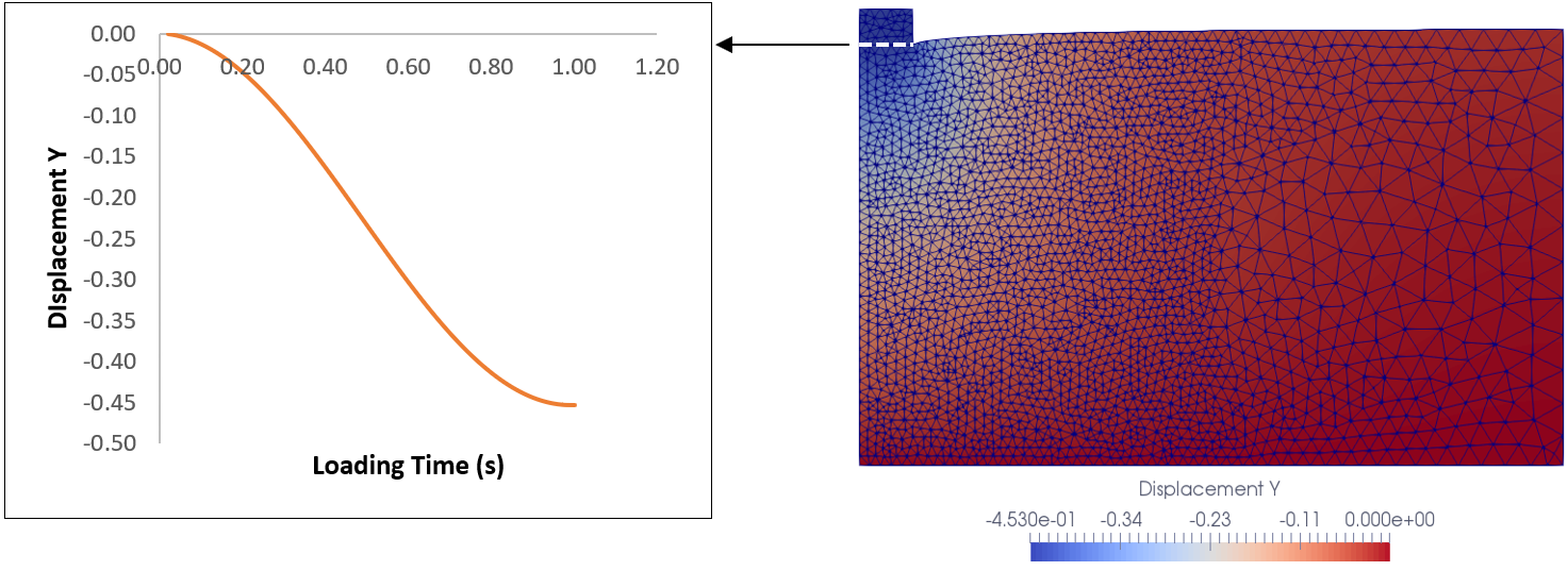
In this example, a simplified case of footing settlement model is considered. A concrete is prescribed with normal surface loading, which is then transferred to underlying soil material. Based on the evolution of Displacement_Y, we consider inversion for material parameters (parameters within Material_data structure) Young's modulus and Poisson's ratio. Three different inversion cases are considered.

 

Target solution retrieved from the surface of interest

 

 

 

GeoInv_002: Pulse decay experiment

 

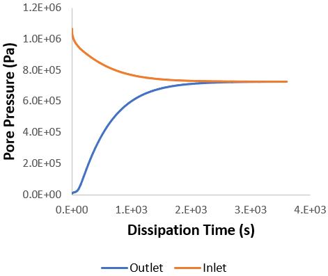
A tight core sample is put into a pulse-decay experiment by flowing helium gas under pressure gradient. The purpose is to recover the equivalent permeability and Klinkenberg slippage factor. As simulation runs, the pressure on the inlet declines while the pressure on the outlet ascends. The change in pressure stops when pressure equilibrium is attained across the core sample. The related data structure is Fluid_properties.

 

Pressure changes towards equilibrium

 

Pressure distribution over time across core sample

 

 

 

GeoInv_003: Fracture stiffness

 

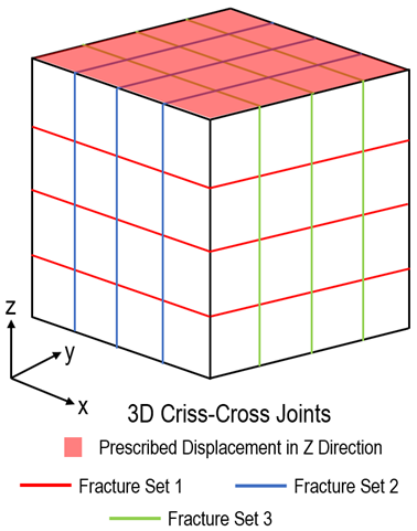
A 3D continuum model is embedded with 3 fracture sets that form criss-cross pattern. The purpose is to recover the initial fracture normal stiffness of each fracture set, as defined in (nonlinear) Bandis model. The related data structure is Fracture_data.

 

Unlike the previous two cases, the use of Tag_name keyword is introduced in this example as an alternative to directly specifying related property data structures (e.g. Material_data).

 

Continuum model embedded with criss-cross joint set

 

 

 

MEM_003: Boundary Optimisation and Super Element in a MEM problem

 

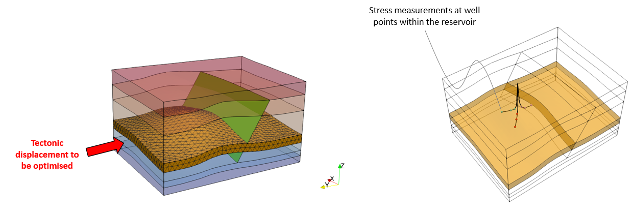
You can find MEM_003 example within the ParaGeo Tutorial Examples section of the manual. Such example demonstrates the usage of the inversion analysis for boundary displacement optimisation within a MEM workflow. To this end reservoir stress measurements at three wells are used as the target solution for the inversion analysis. Cases with and without the Super Element approach are demonstrated.

 

Displacement optimisation MEM_003 example case