ParaGeo Tutorial Examples

Contents
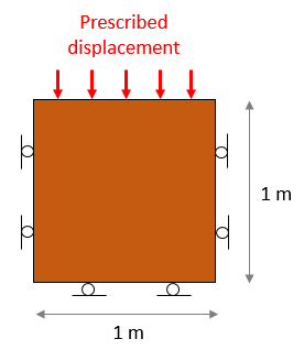
Welcome to the ParaGeo tutorial examples manual chapter. Here the user will encounter several practice examples specially designed to learn the usage of the main ParaGeo functions. In each example the definition of several key data structures are discussed and an example datafile is provided. It is recommended for the user to go through this examples defining his own datafile in order to improve and consolidate the model definition using ParaGeo data structures.
INDEX
Title |
Analysis Type - Features List / Utility |
Model |
Introduction |
||
Mechanical (2D) |
|
|
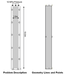
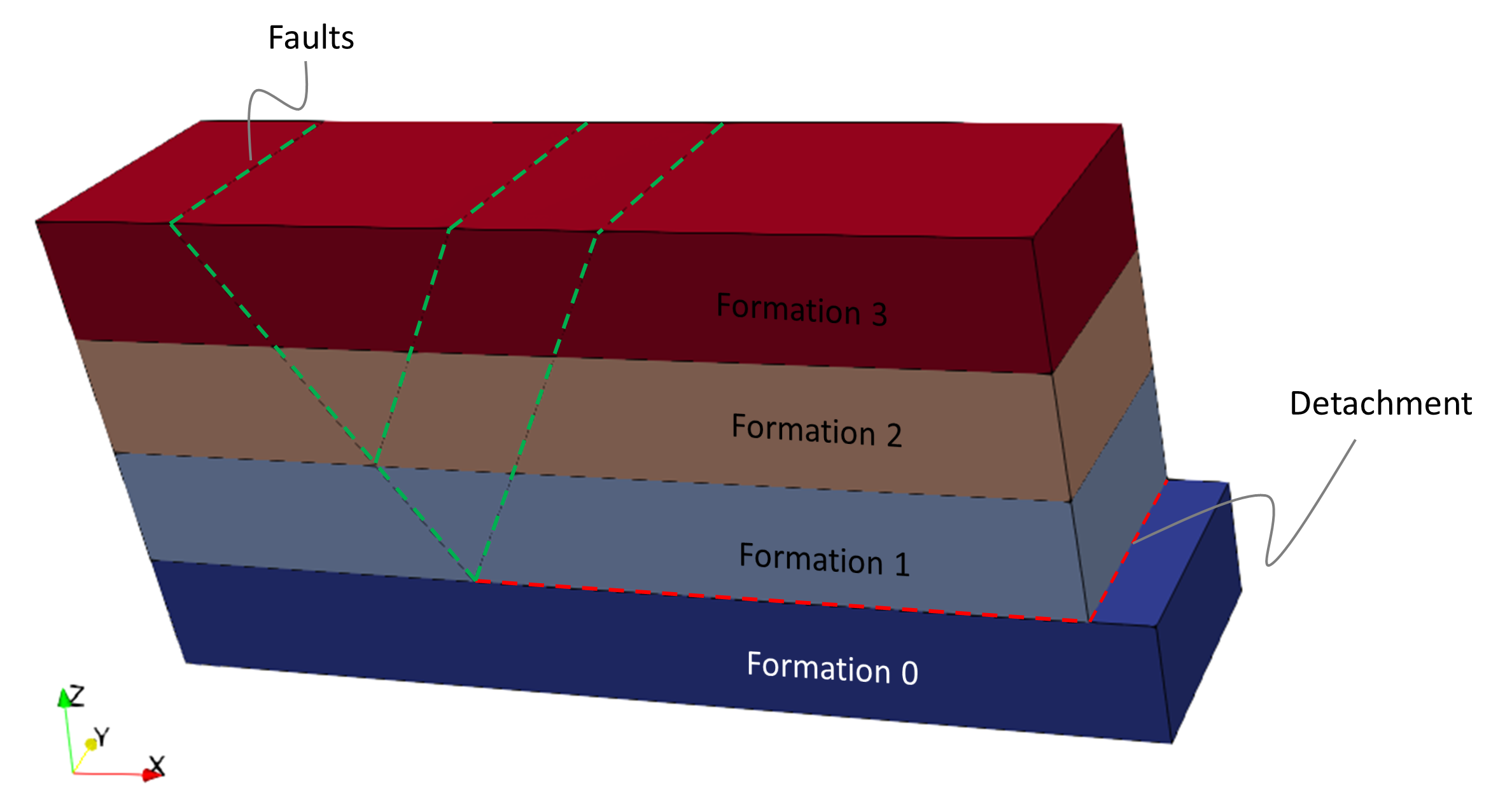
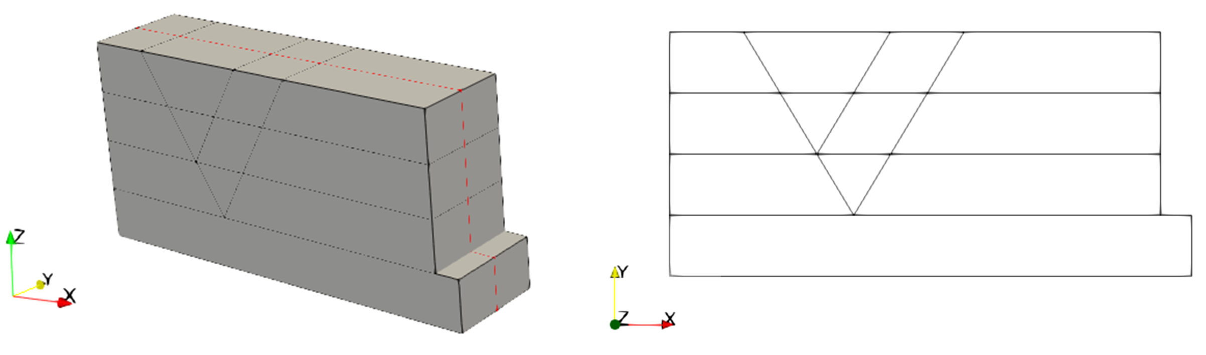
•Defining model geometry data |
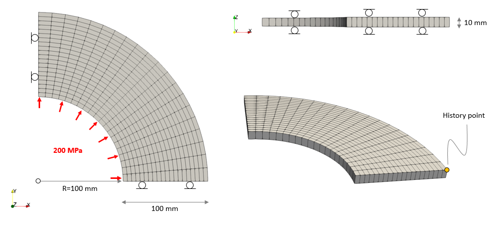
Model geometry and boundary conditions |
|
•Parageo groups •Defining model geometry sets |
||
Mesh Generation |
||
Mesh Generation (2D) |
|
|
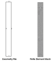
•Mesh discretization for various models with different geometry entities
|
|
|
|
||
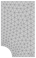
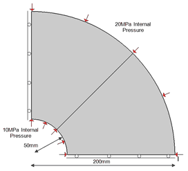
•Case 1C Plate with Hole Plate with Hole (Quadratic Lines with Mesh Refinement) |
||
•Case 1D Plate with Hole (Mesh Refinement using Mesh Region) |
||
|
||
Mesh Generation in ParaGeo (3D) |
|
|
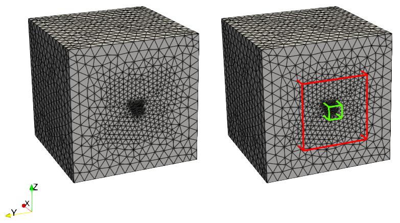
•Approach to export a generated mesh in a .geo file •Definition of element sizes using different strategies •Usage of adaptivity for more flexibility |
|
|
•Case 03 Usage of adaptivity with regions of different element sizes |
||
Mechanical Analysis |
||
Mechanical (2D) |
|
|
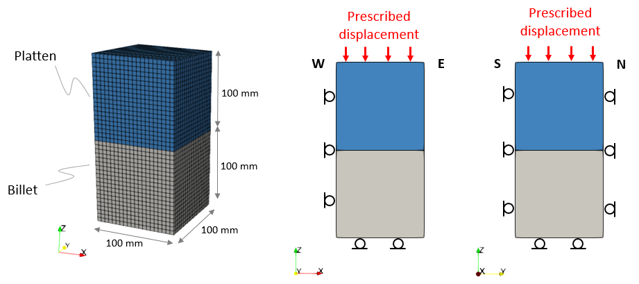
•Case 1A Base Case Description •Case 1B Scaling Time for 100 Steps •Case 1C Scaling Time for 1000 Steps •Case 1F Instantaneous Loading
|
•Explicit dynamic solver •Various strategies for quasi-static solution •Time scaling •% Global damping •Various time curves - linear, nonlinear, instantaneous
|
|
|
||
Mechanical (2D) |
|
|
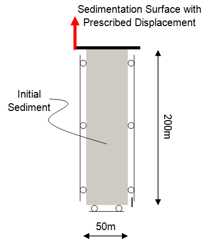
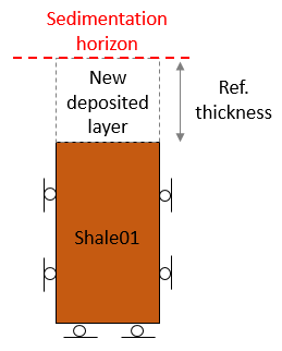
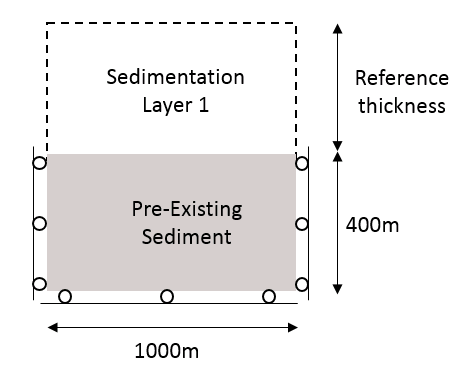
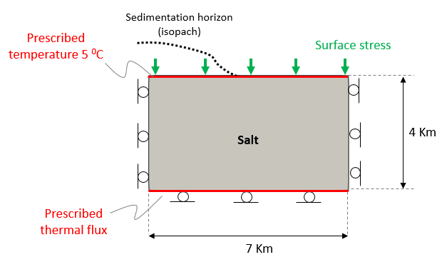
•Constant/Variable sedimentation
|
|
|
Mech_003 Rift Sandbox Simulation using Prescribed Boundary Data |
Mechanical (2D) |
|
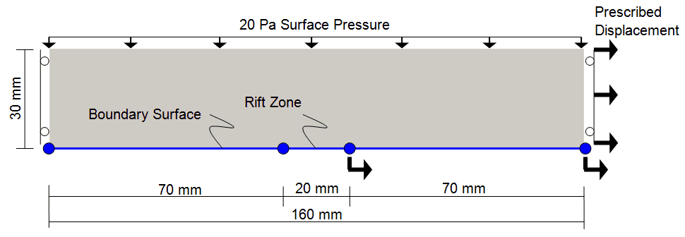
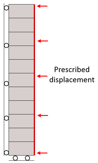
•Case 1 Extension via a Prescribed Boundary |
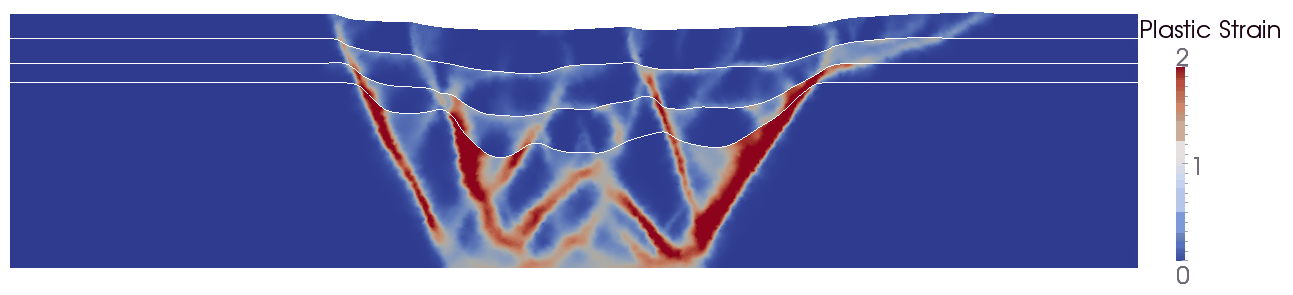
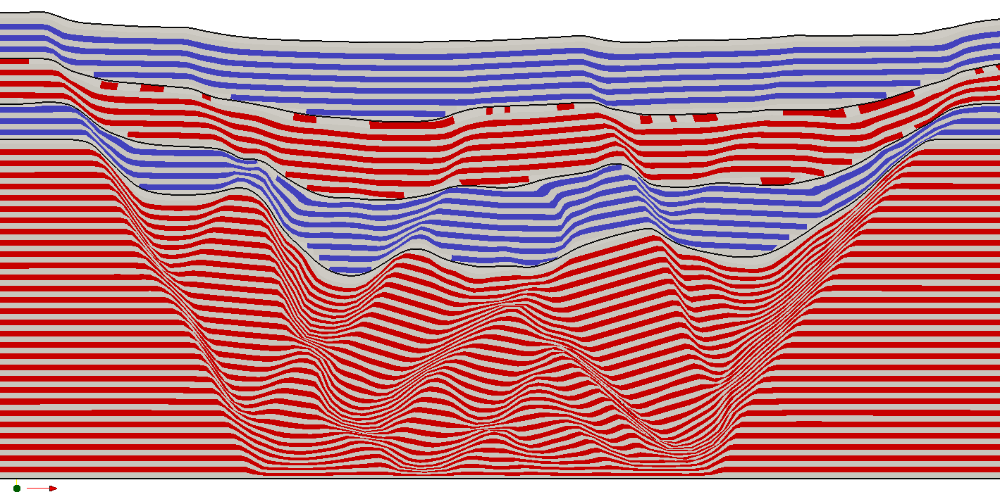
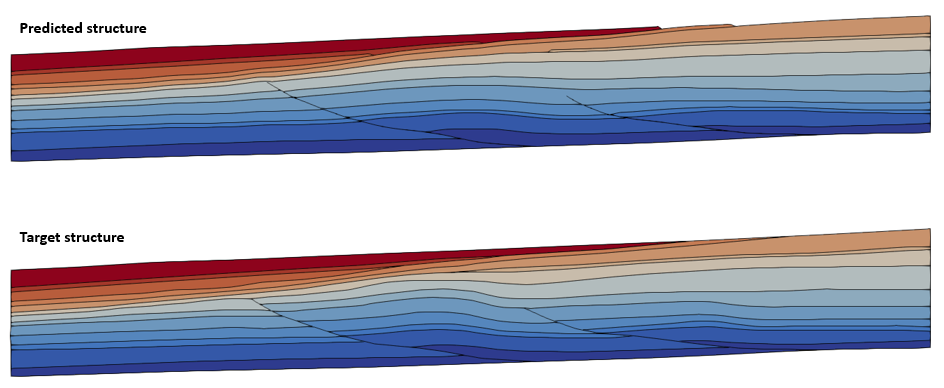
•Multi-layer sedimentation •Stratigraphy definition •Material grids •Adaptive mesh refinement with coarsening data and plastic strain rate •Prescribed boundary displacement using part-geometry and prescribed boundary data |
|
Mechanical (2D) |
||
•Case 1 Basic Set Up for Adaptive Remeshing |
•Adaptive mesh refinement with coarsening data and plastic strain rate •Material grids
|
|
Mechanical (2D) |
|
|
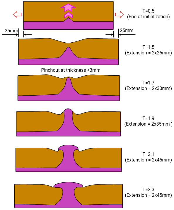
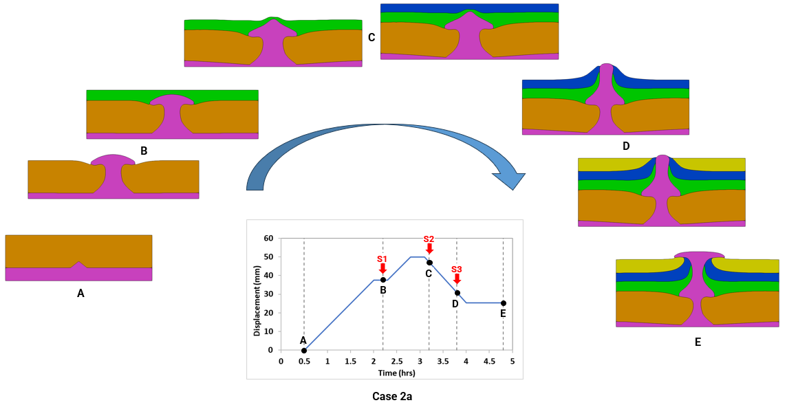
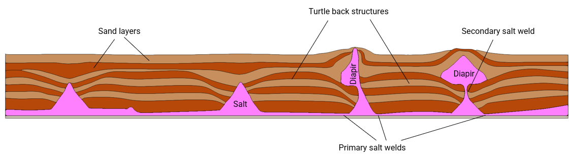
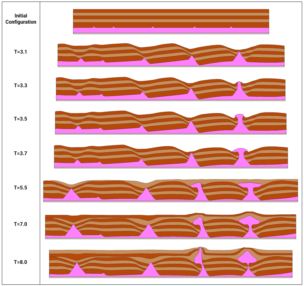
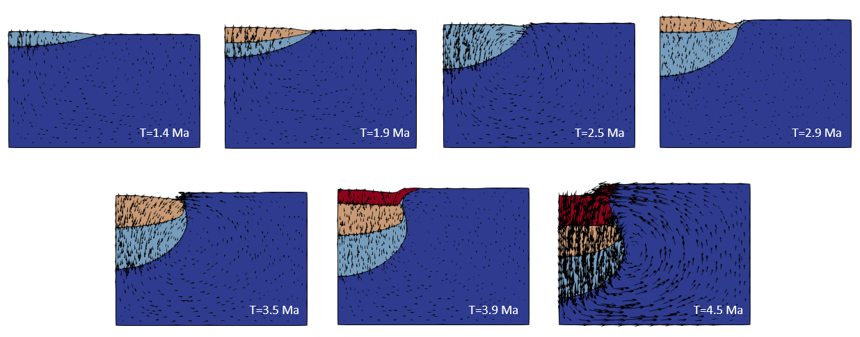
•Salt material modelled with Herschel-Bulkley viscoplastic material model •Sand material modelled with SR4 plasticity model •Extensional/Compressional tectonic movement settings •Layer sedimentation using variable sedimentation rates/fixed sedimentation horizons •Stratigraphy pinchout •Adaptive mesh refinement with coarsening data and strain rates •Single/Multiple seed point/s for diapir/s formation |
|
|
|
||
|
||
Material Models |
||
Mechanical (2D) |
|
|
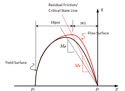
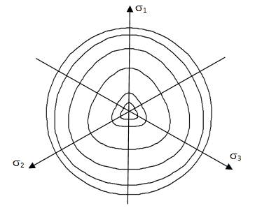
•SR4 material model |
|
|
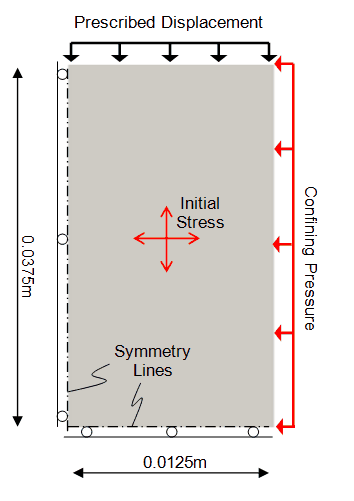
•Case 1 Simulation of Triaxial Tests with the SR4 model •Case 2 Characterization of Experimental Data with the SR4 Model (Linear Elasticity) •Case 3 Characterization of Experimental Data with the SR4 Model (Poroelasticity) |
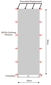
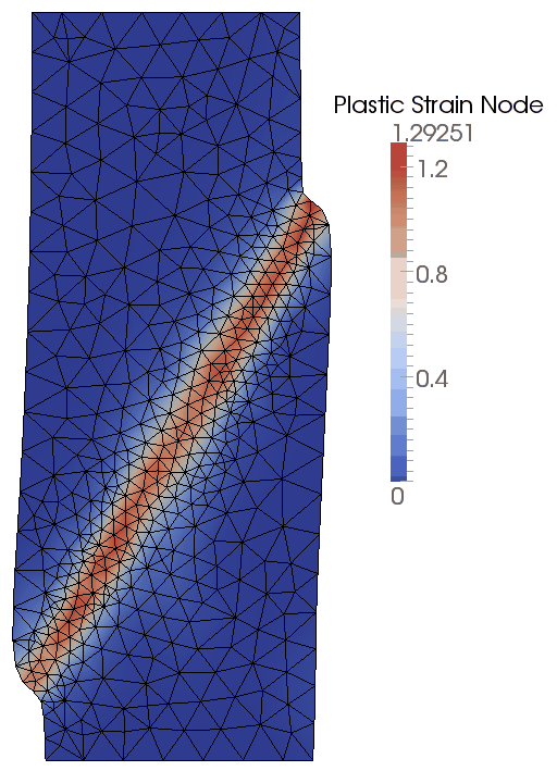
•Triaxial tests •Material characterization of experimental data for SR4 model with linear elasticity/poroelasticity |
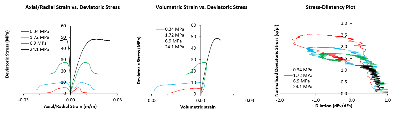
Plots from experimental tests |
Mechanical (2D) |
|
|
•SR4 material hardening parameters and calibration of kappa and lambda using SR4 analytical model |
|
|
Mechanical (2D) and Coupled THM (2D) |
|
|
•SR4 material hardening calibration to user-defined hardening model •Provision of facies mixture-based material database spreadsheet and step by step description for user-derivation •Axi-symmetric single element oedometer test (geomechanical) •Uniaxial column consolidation test (coupled THM) |
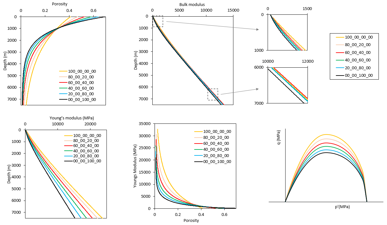
Mechanical properties for different component % of Sandstone, Siltstone, Shale, Carbonate (Ss_Si_Sh_Ca) |
|
Mechanical (2D) and Coupled THM (2D) |
|
|
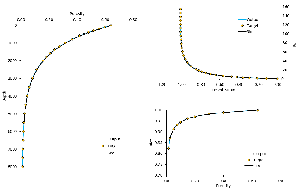
•Simplified input of data in the form of Athy-type models to characterise mechanical compaction •Automated hardening data generation |
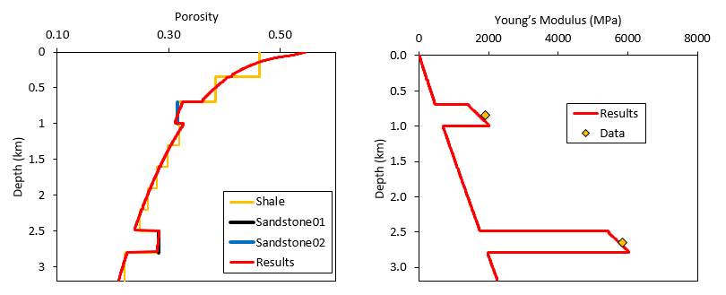
Validated results generated using the mechanical compaction models |
|
Mechanical (2D) |
|
|
|
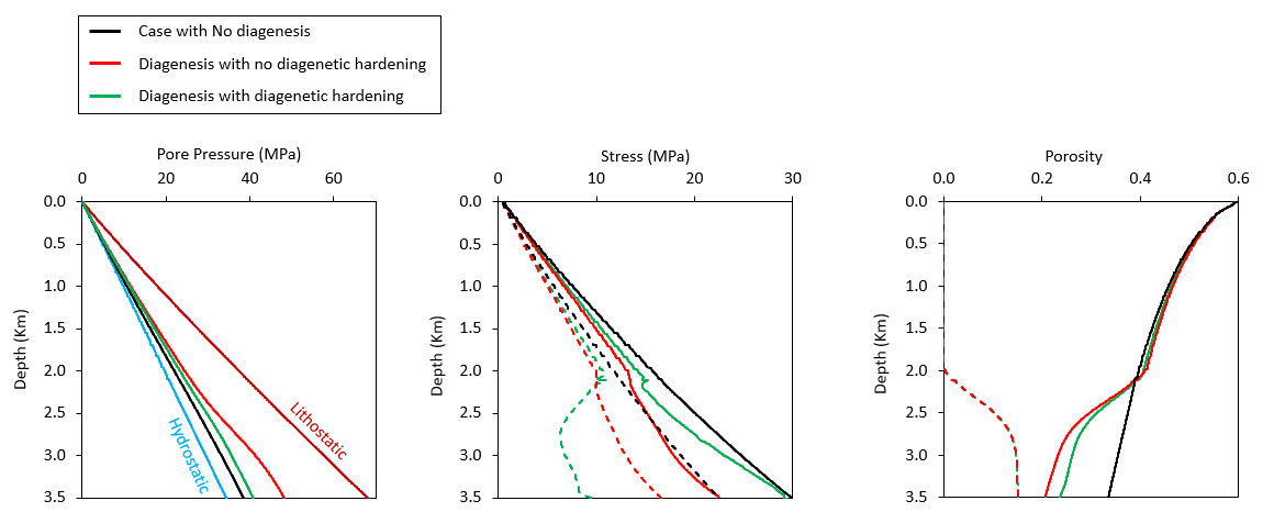
•Diagenesis model and behaviour
|
|
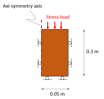
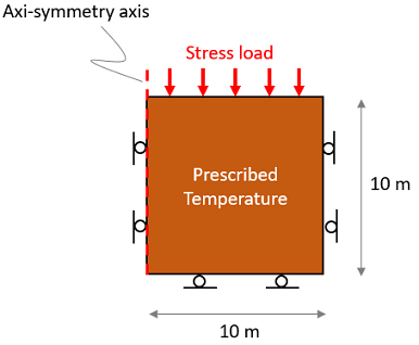
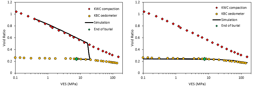
•Calibration of diagenesis law for Kimmeridge Clay and Berea Sandstone •Axi-symmetric single element oedometer test/burial history simulation |
Axi-symmetric single element: Oedometer test (left), Burial history simulation (right)
Results vs geomechanical tests. Simulation of burial history (left). Additional unloading/reloading (right) |
|
Mat_003 Continuum Fracture Model (PVC test on a fractured specimen) |
Coupled HM (3D) |
|
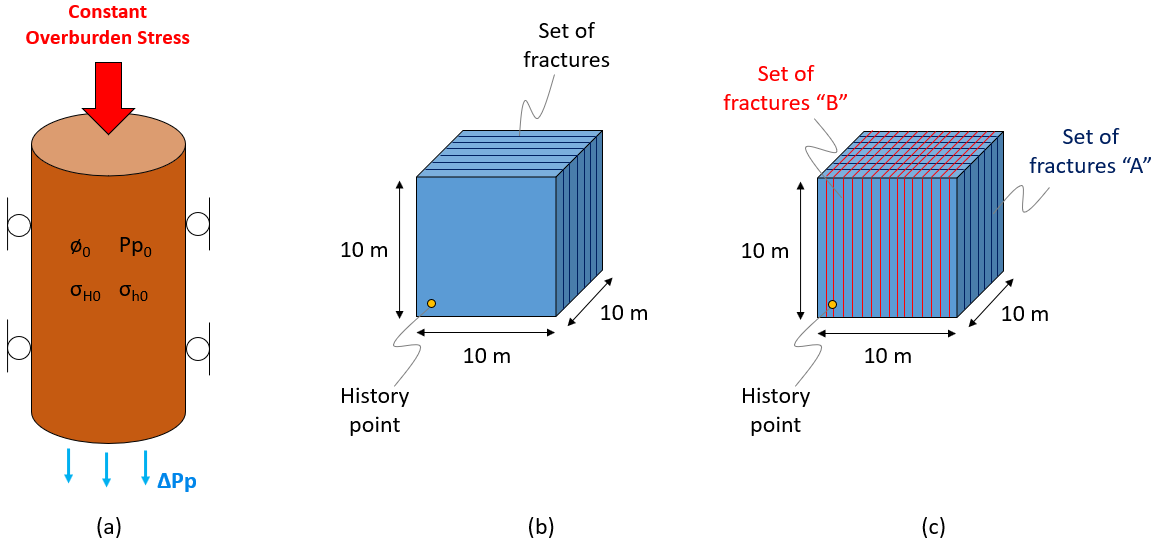
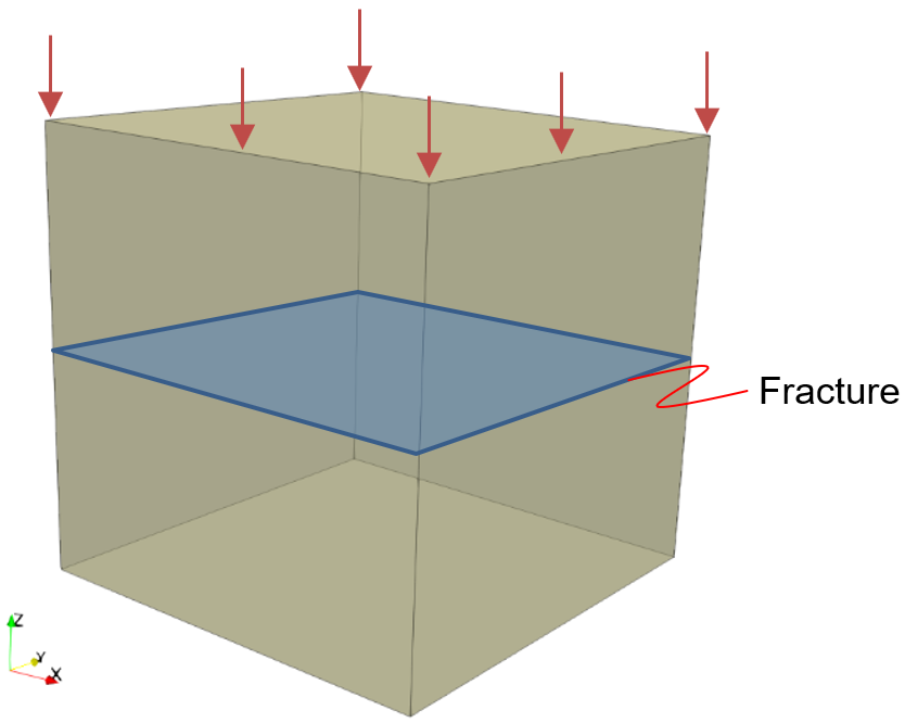
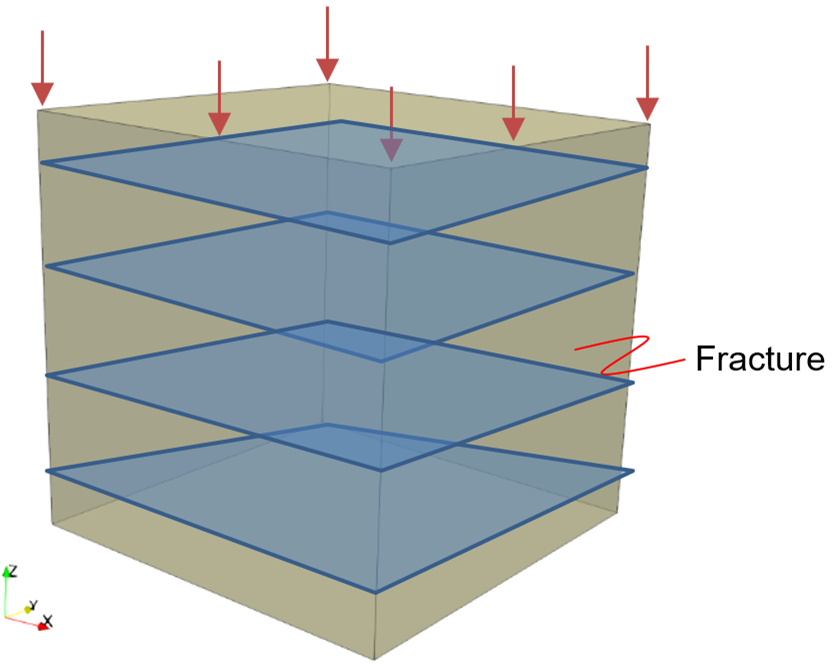
•Case1a Poroelastic simulation •Case1b Poro-elasto-plastic (SR4) simulation •Case 2a (poroelastic) and Case 2b (SR4) with 2 sets of fractures |
•Pore Volume Compressibility (PVC) test •Poroelastic / with SR4 plasticity materials •Single hex element continuum fracture model with one/two fracture sets |
(a) Schematic of PVC test, (b) Model with 1 fracture set (Case 1), (c) with 2 fracture sets (Case 2) |
Mechanical (2D) |
|
|
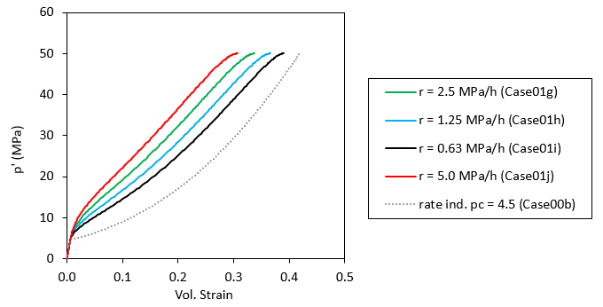
•Case02 Power law model with accelerated creep at high deviatoric stresses |
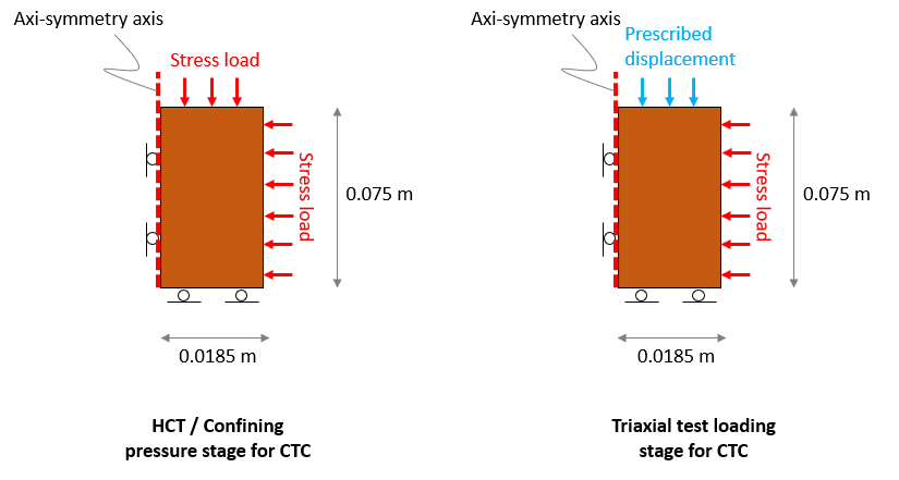
•SR3 plasticity model with simple Power law creep/Power law with accelerated creep at high q •Hydraulic Compression Tests (HCT) and Triaxial tests (CTC) at different loading rates |
|
Fracture Models |
||
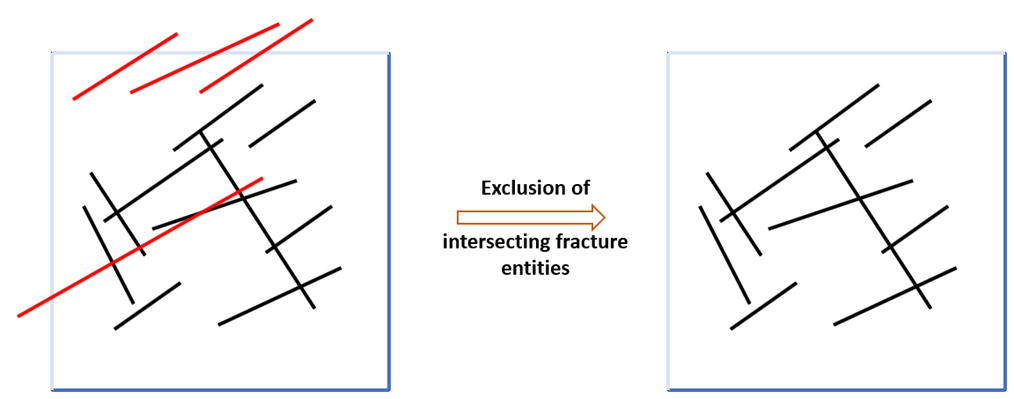
•Overview of the representation of fractures in ParaGeo •Features and considerations on the fracture import workflow |
|
|
Coupled HM (3D) |
|
|
•FracMan File (.fab) Description •Case00 Import of the FracMan DFN for Visualisation Only •Case01 Import, Processing and Export to a New FracMan File •Case02 Import, Processing, Meshing and Export to a .geo file |
•ParaGeo fracture data import/export from/to FracMan data •Export of processed DFN to new FracMan file •Export of the meshed geometry with the DFN to a .geo file
|
|
Coupled HM (3D) |
|
|
|
•Discrete fracture modelling with FracMan imported data |
|
Mechanical (3D) |
|
|
•Case01 Joint Normal Displacement with Bandis Model •Case02 Joint Normal Displacement with Bandis Model (Spacing 0.25m) |
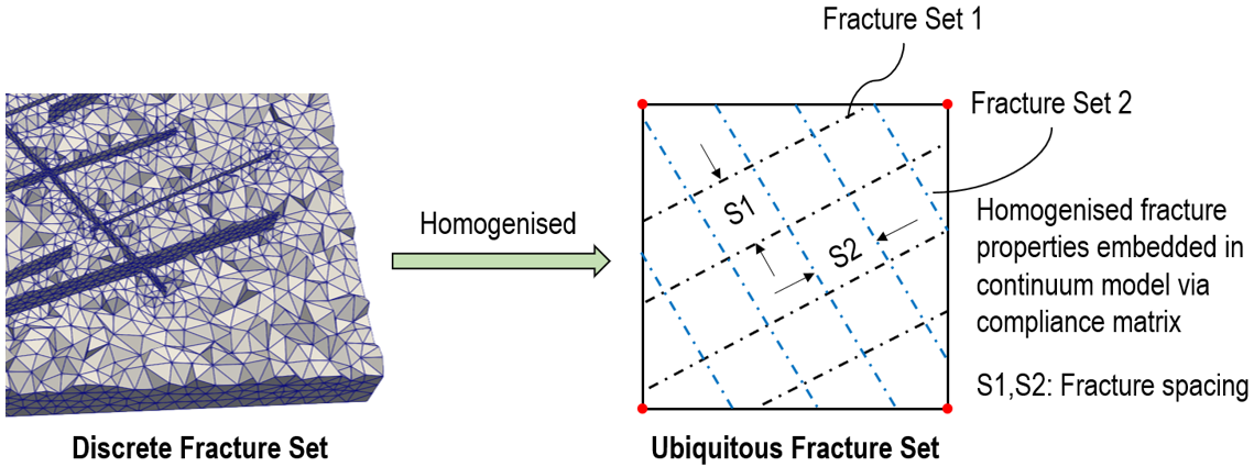
•Embedded continuum fracture modelling using Ubiquitous Element Fracture (UEF) approach in mechanical field •Homogenised fracture properties via compliance matrix •Bandis fracture normal stiffness model •Normal displacement loading |
|
Fract_004 Homogenisation of Flow Properties in Jointed Model |
Coupled HM (3D) using ParaGeoInv |
|
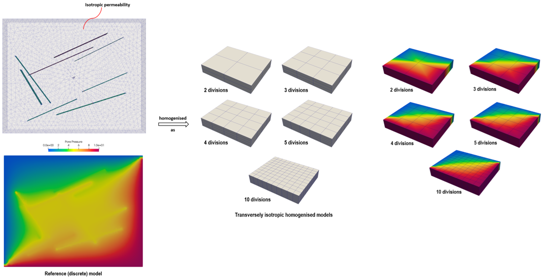
•Case01 Ubiquitous Upscaled Fracture (UUF)
|
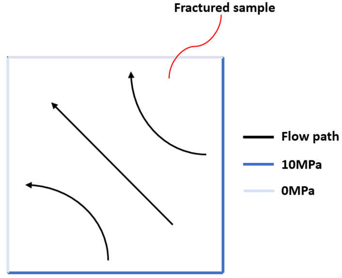
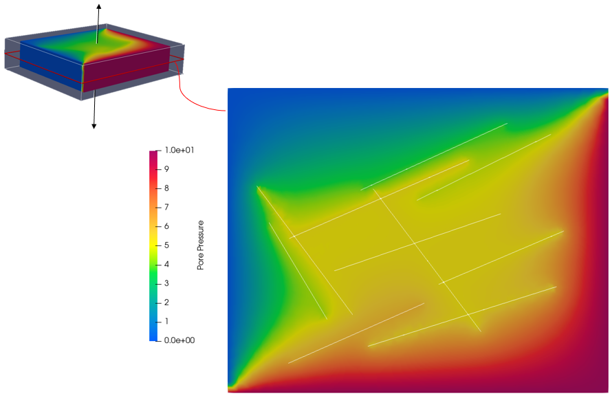
•Homogenisation of flow properties (e.g. material permeability) using Ubiquitous Upscaled Fracture (UUF) approach
|
|
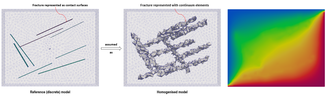
•Homogenisation of flow properties (e.g. fracture permeability multiplier) using Spatially Embedded Fracture (SEF) approach |
|
|
Hydro-Mechanical Coupled Analysis (HM) |
||
HM_001 Introduction to Hydro-Mechanical Analysis - Uniaxial Consolidation |
Coupled HM (2D) |
|
|
•Coupled HM data definition •Uniaxial consolidation (no gravity) |
|
Coupled HM (2D) |
|
|
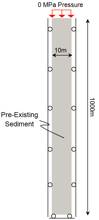
•Base Case 1 Permeability = 1E-18 m2 |
•Coupled HM data definition •Uniaxial consolidation with gravity •Various permeabilities •Sedimentation time curve types (linear/s-curve) |
|
HM_003 Uniaxial Sedimentation using Eulerian Deposition (Currently unavailable) |
Coupled HM (2D) |
|
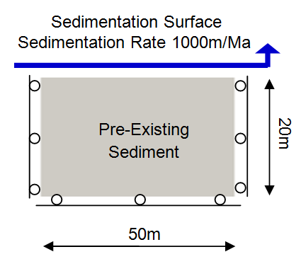
•Case 2 Permeability = 1E-19 m2 |
•Uniaxial sedimentation using Eulerian deposition •Moving Eulerian deposition surface defined using part geometry data and prescribed boundary data •Various permeabilities •Sedimentation time curve types (linear/s-curve) |
|
Coupled HM (2D) |
|
|
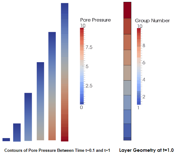
•Uniaxial sedimentation using layer deposition •Stratigraphy data •Sedimentation data
|
|
|
HM_005 Uniaxial Sedimentation using Layer Deposition Followed by Tectonic Compression |
Coupled HM (2D) |
|
•Stage 1 uniaxial 'drape' sedimentation using layer deposition •Stage 2 tectonic compression at various strain rates •Restart data definition for stage 2 simulation
|
Stage 1 - Drape sedimentation (left), Stage 2 - Tectonic compression (right) |
|
Thermo-Hydro-Mechanical Coupled Analysis (THM) |
||
Coupled THM (3D) |
|
|
|
•Coupled THM data definition •Contact data with heat and fluid flow across contact surfaces |
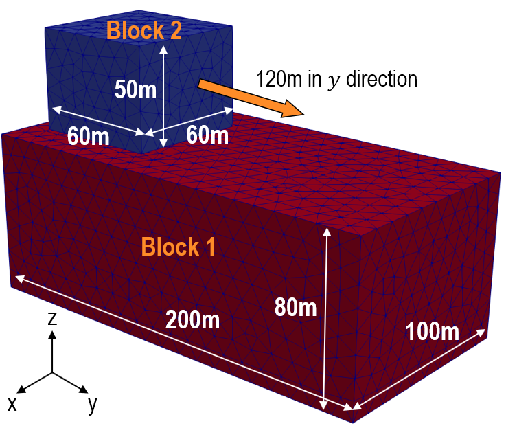
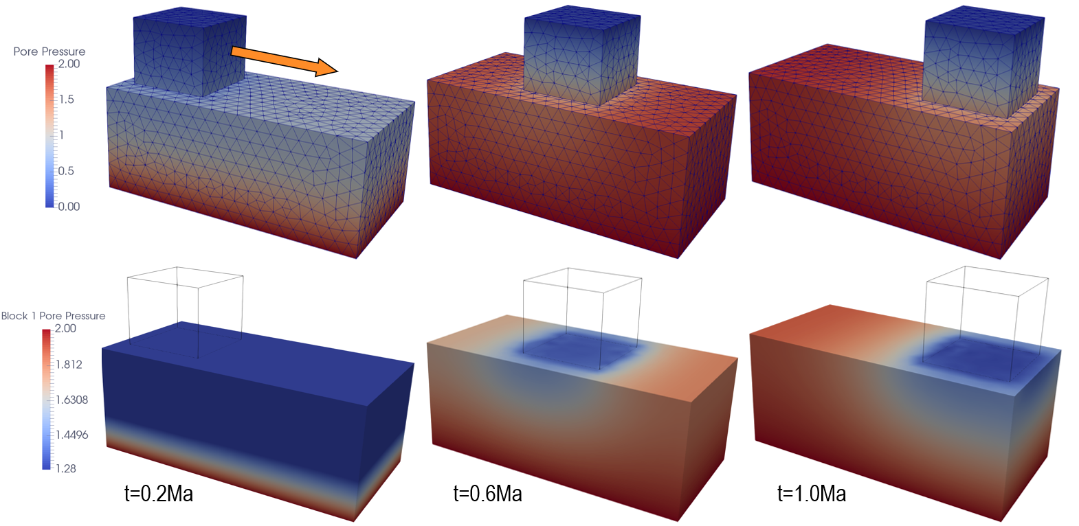
Geometry description (left), Pore pressure distribution due to movement of fluid sink (right) |
Contact |
||
Mechanical (3D) |
|
|
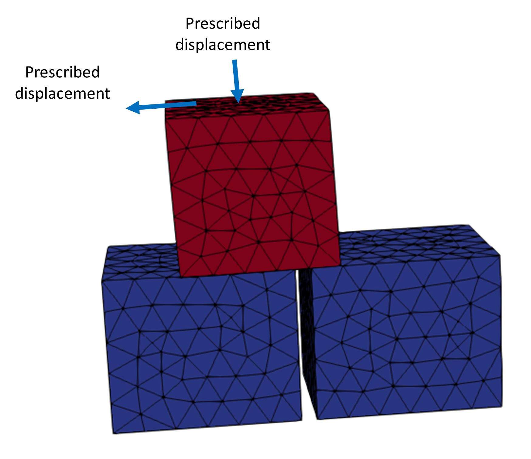
•Mechanical contact data definition •Various contact models (adhesion, with/without slip, penetration dependent stiffness) |
|
|
Coupled THM (2D) |
|
|
•Case 1 Constant contact properties for fluid and thermal contact •Case 2 Contact tangential permeability as a function of stress •Case 3 Contact tangential permeability as a function of depth |
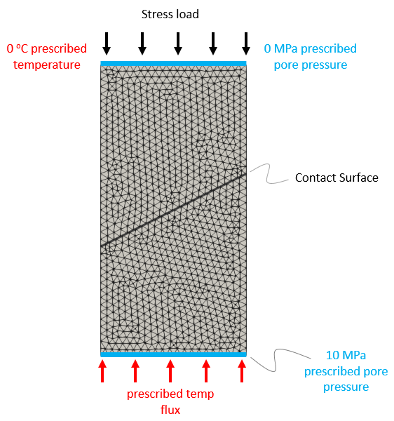
•Coupled THM data definition •Contact data with heat and fluid flow across contact surfaces •Various contact flow models |
|
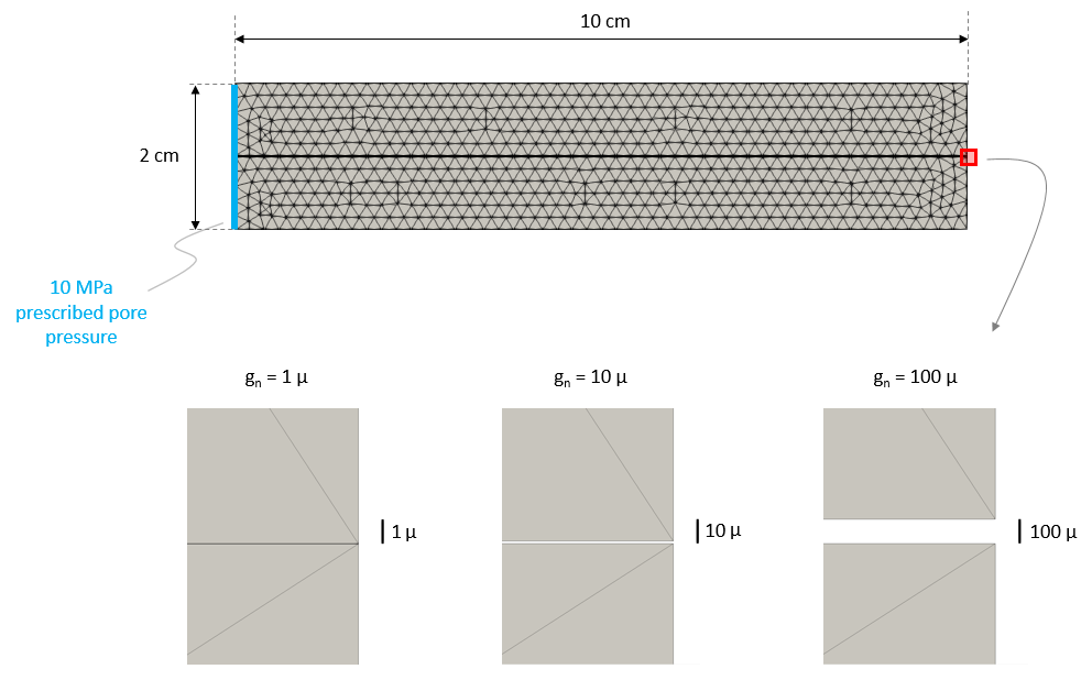
•Case 4 Contact tangential flow conductivity as a function of contact gap |
•Contact tangential flow model as a function of actual contact gap |
|
Mechanical (3D) |
|
|
•Case01 and Case02 Comparison of node-to-node and node-to-facet contact algorithms |
•Comparison of contact algorithms (node-node vs node-facet) |
|
Spatial Variation |
||
SpatVar_001 Definition of properties with spatial variation (via Grids) |
Mechanical (2D & 3D) |
|
•Case1 Base Case Description (Grid type 1) •Case1b Base Case grid defined at cell centres •Case2 Definition of grid type 3 (equivalent to Case1 grid) •Case3 Definition of non-regular cells grid (Grid type 3) •Case4 Usage of Spatial table (property dependencies) •Case5 Spatial plan (lateral variation in properties) |
•Different spatial grid types (Grid1, Grid3, Plan1, Group) •Definition of variables at nodes/elements •Spatial table for defining variables with dependencies on other variables •Spatial plan data in 2D for lateral property variation •Spatial grid group data (mesh based) •Spatial boundary grid mapping options for points outside grid |
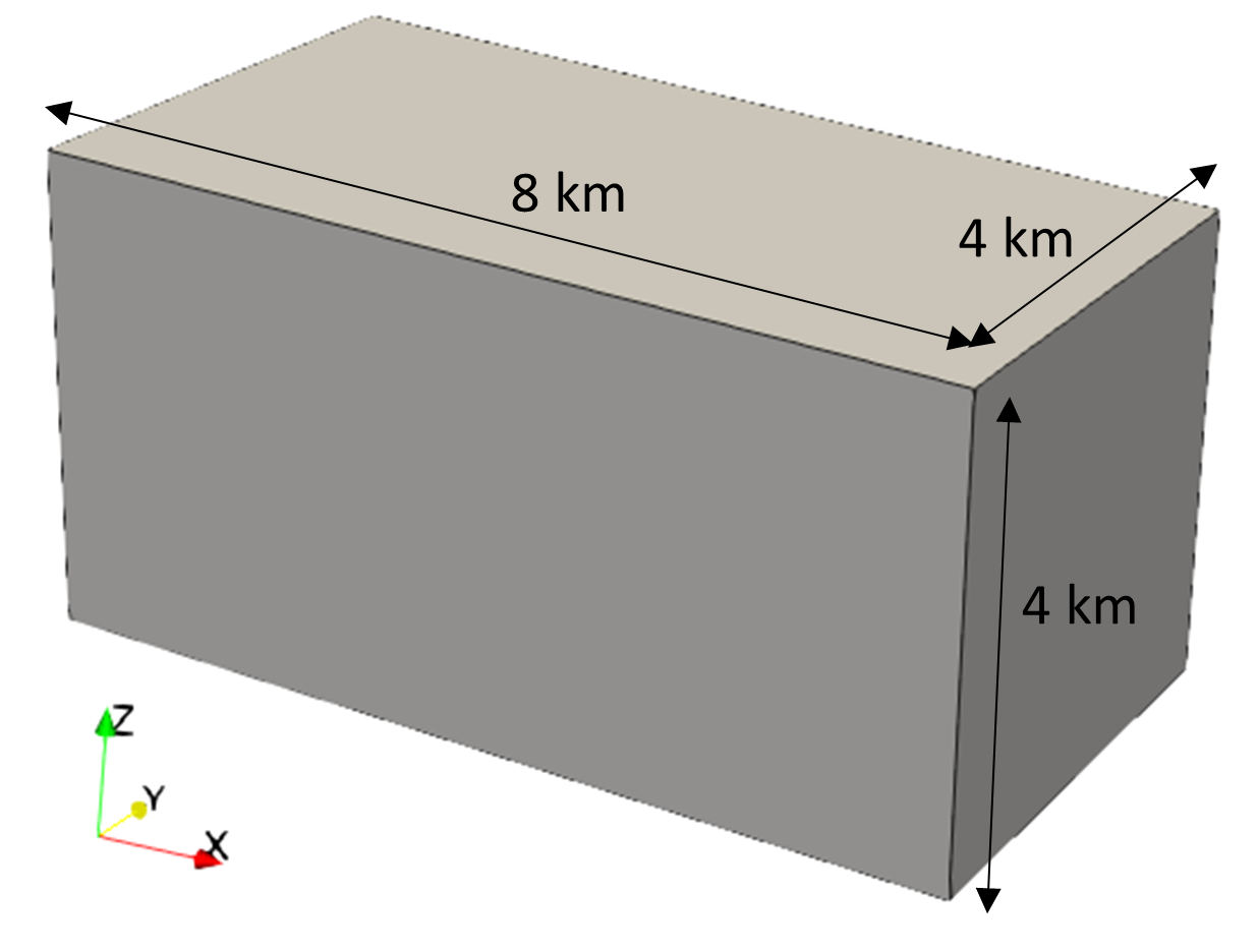
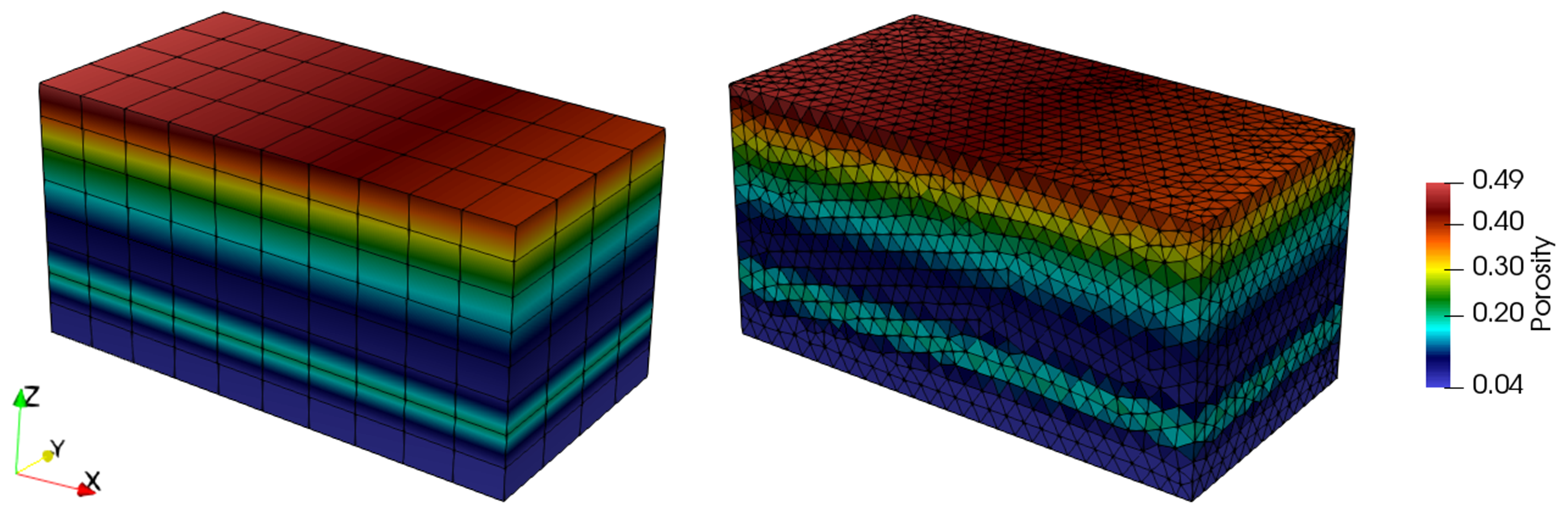
Geometry (top), Defined spatial grid (left), Mapped mesh variable (right) |
Mechanical (2D) |
|
|
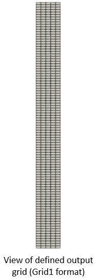
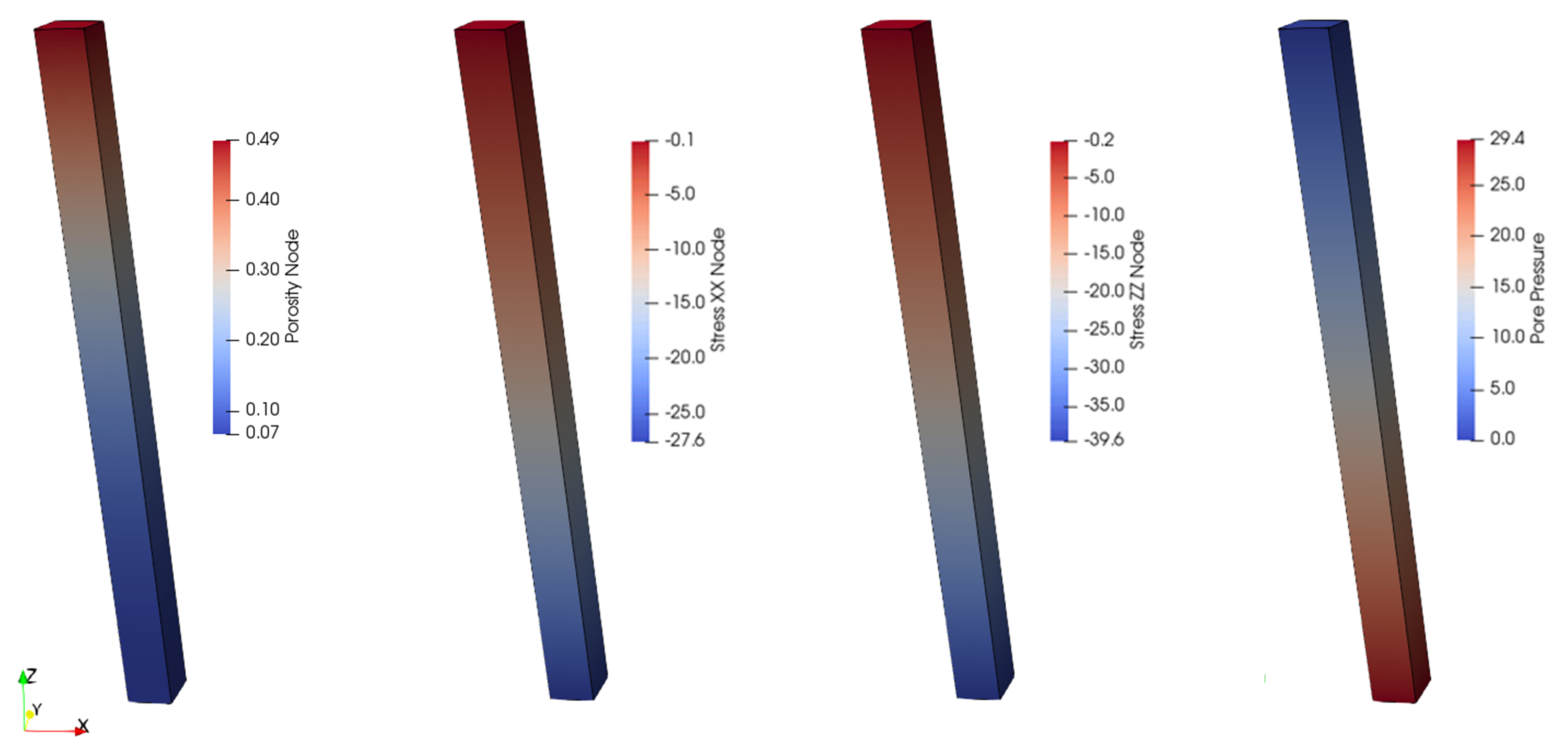
•Case1 Base Case Description (Output of Mesh Grid) |
•Output of results to spatial grids with different grid formats (Group, Grid1) •Definition of reference set data to output change in specified variables and export to spatial grids
|
|
Geostatic Initialization |
||
Coupled HM (3D) |
|
|
•Case 2 Over-consolidated porosity trend •Case 3 Displacement reinitialization •Case 4 Initialization with initial overpressure (via spatial grids) |
•Gravity loading •Geostatic initialization •Initial porosity depth trend defined via spatial variation data •Initial pore pressure defined as hydrostatic or via spatial grid .spat file •Usage of staged geostatic control data for displacement reinitialization |
|
Mechanical (3D) |
|
|
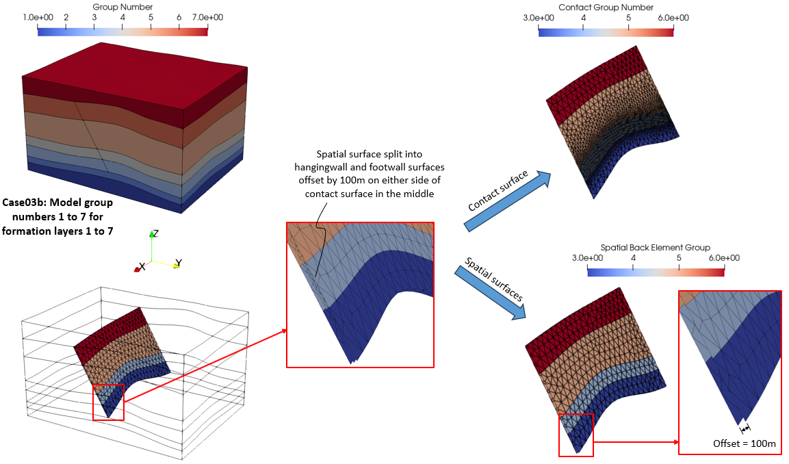
•Case 1 Base Case Description (Elastic Initialization) •Case 3 Switch to standard models •Case 4 Displacement Reinitialization •Case 5 Porosity Initialization via Spatial Grids |
•Faulted model with contact •Gravity and tectonic loading •Geostatic initialization •Initial porosity depth trend defined via spatial variation data/spatial grid .spat file •Young's modulus - porosity dependent spatial table •Usage of staged geostatic control data for displacement reinitialization, switching constitutive and contact models •Usage of geostatic.set for staged geostatic control data |
|
Sub-Modelling |
||
Mechanical (3D) |
|
|
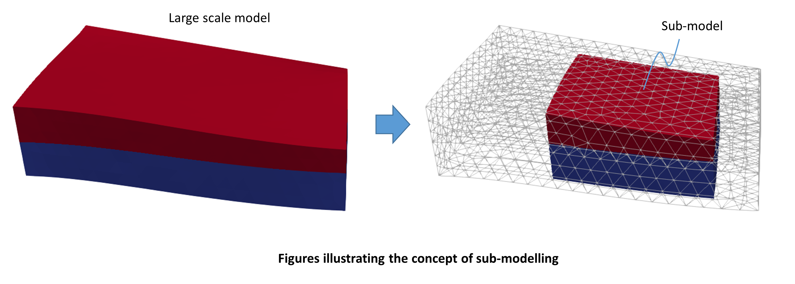
•Step 2 Sub-model Boundary Creation |
•Sub-model boundary export definition to spatial grids •Spatial grid mapping •Prescribed boundary conditions using Spatial boundary data |
|
Restoration |
||
Mechanical (2D) |
|
|
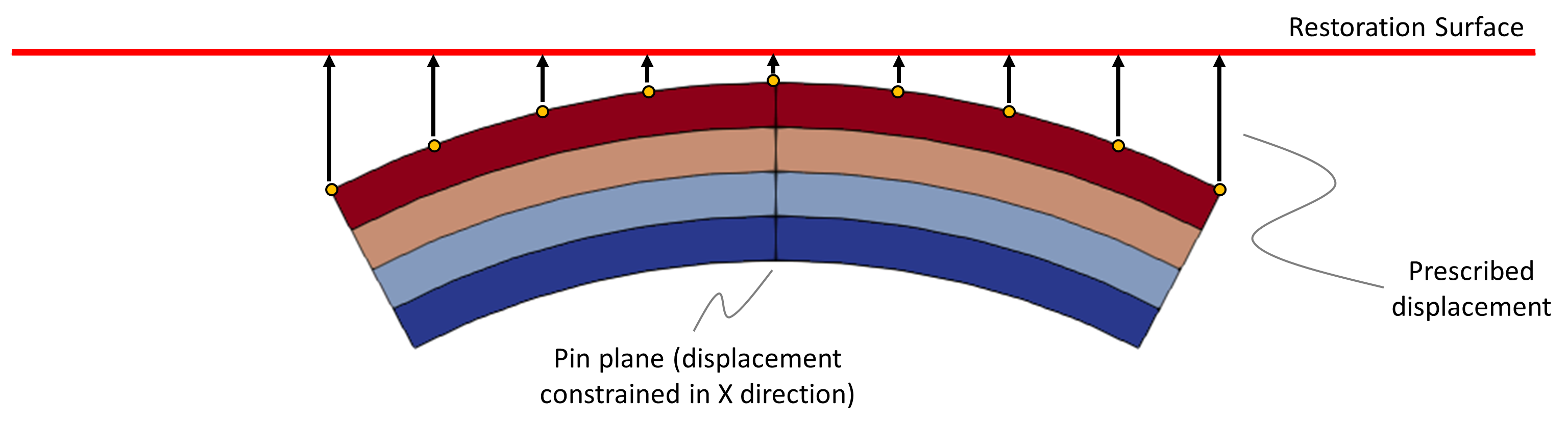
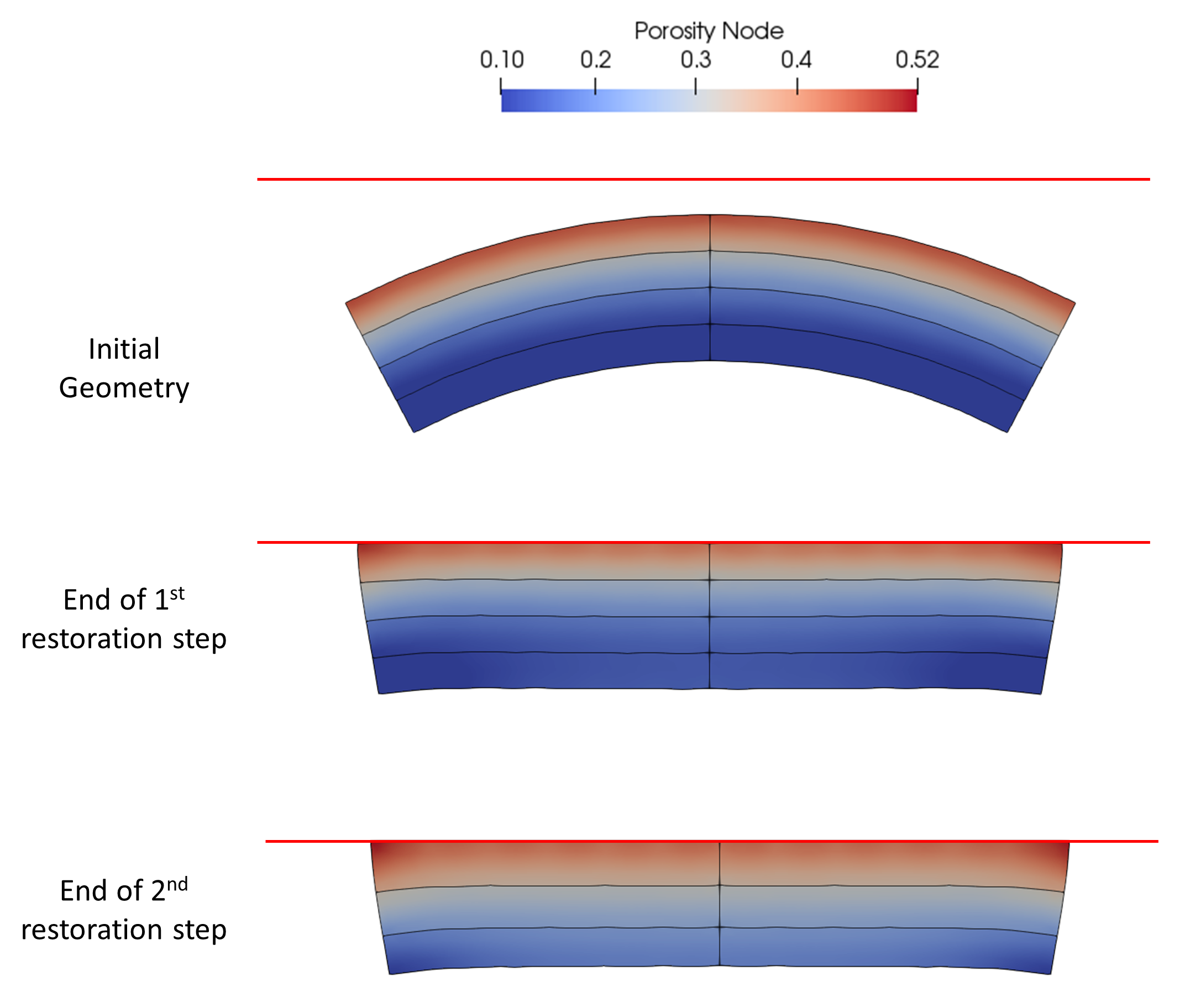
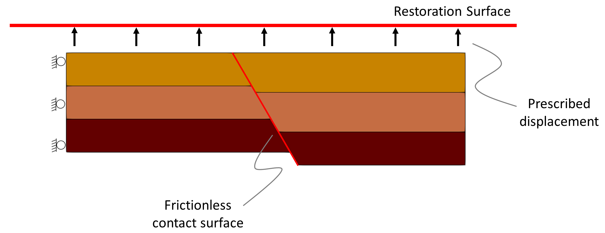
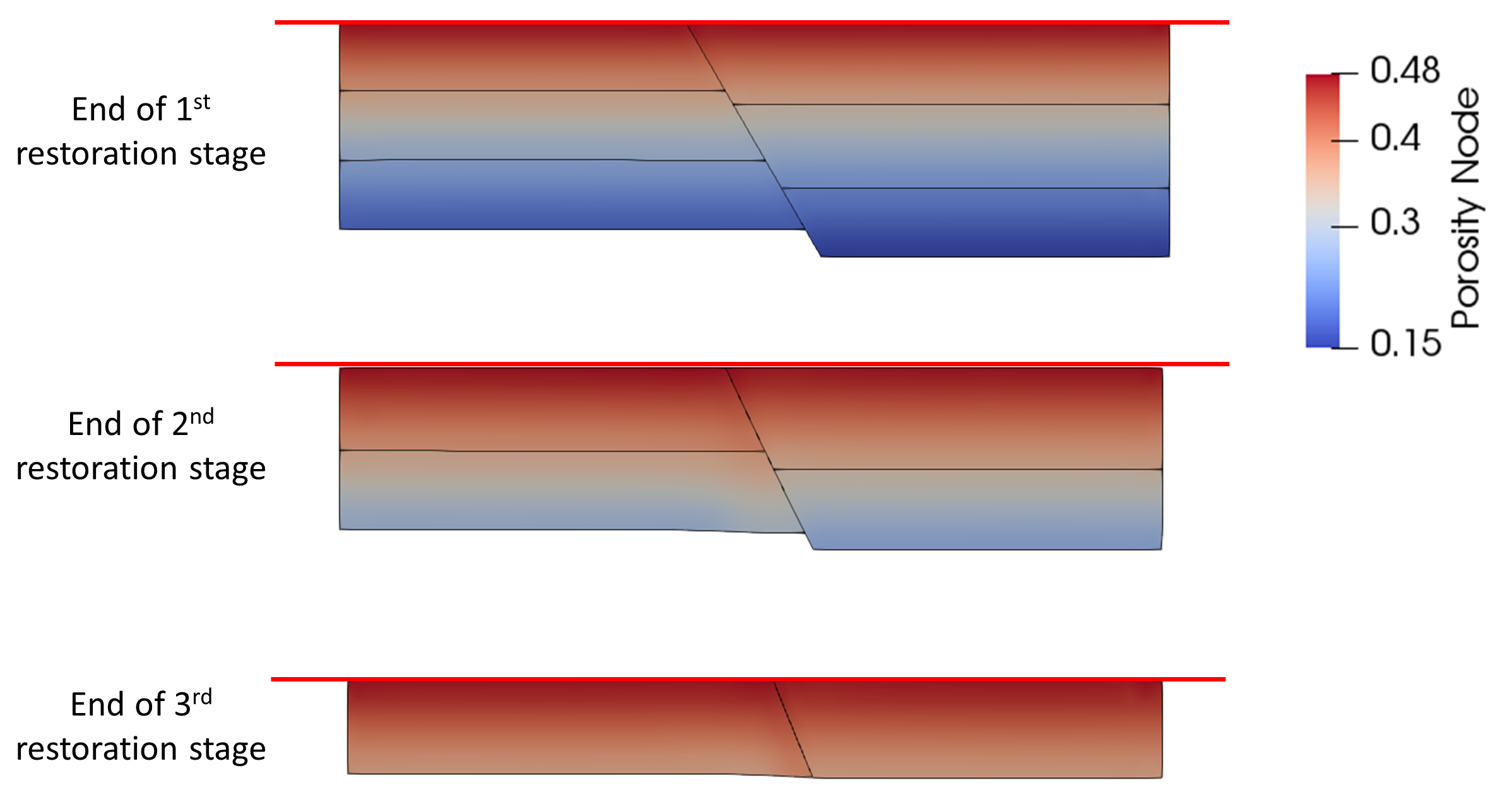
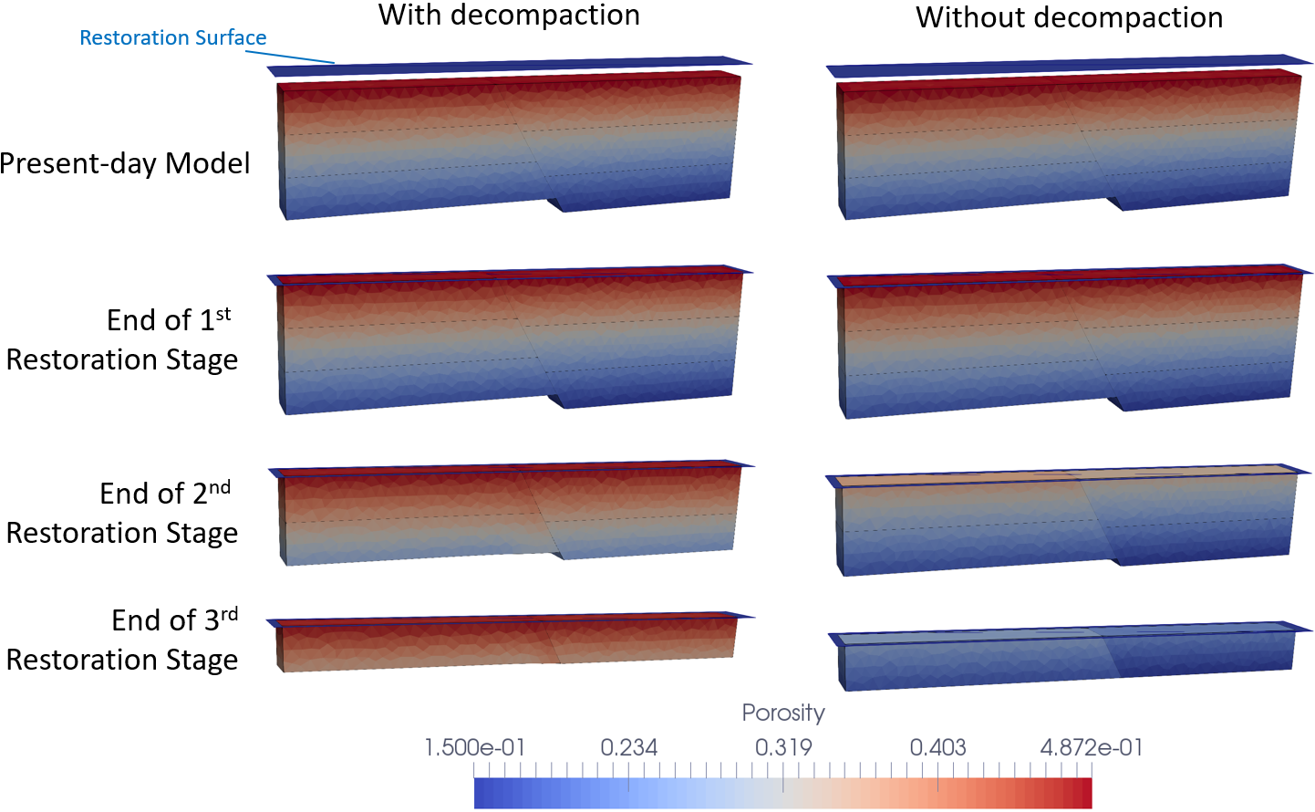
•Case 2 Restoration with Bedding Plane Slip •Case 3 Restoration with Decompaction (Synchronous) •Case 3b Restoration with Decompaction (Sequential) •Case 4 Force-based bed length constraint (High stiffness) |
•Restoration - translate/restore •Restoration with bedding plane slip •Restoration with decompaction following prescribed porosity vs depth trend •Part geometry data •Stratigraphy definition •Top surface bed-length constraint/preservation using force/displacement |
|
Mechanical (2D) |
|
|
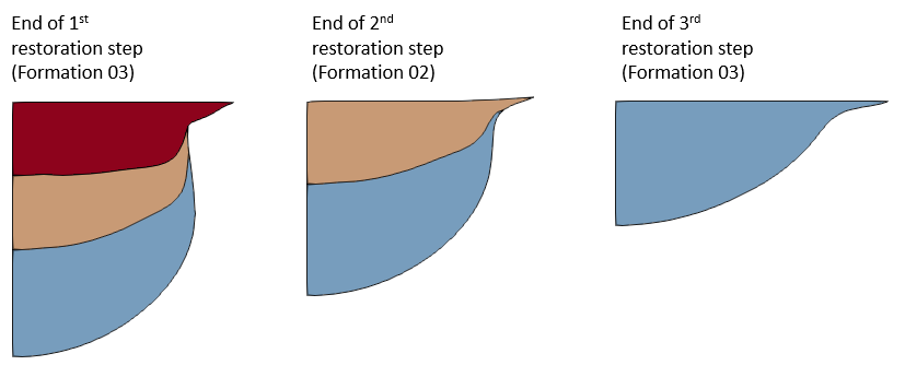
•Step 2 Forward create data file •Step 3 Description of the generated forward simulation data file |
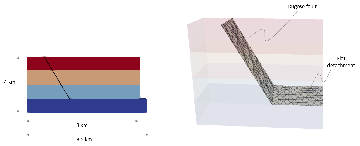
•Faulted model with contact •Restoration with decompaction •Utility to create forward model data from restoration |
|
Rest_002b Restoration to forward: A normal fault model in 3D (Currently unavailable) |
Mechanical (3D) |
|
•Step 1 Restoration
|
•Faulted model with contact •Restoration with decompaction
|
|
Rest_003 Restoration to forward work flow for mini-basin type models (Currently unavailable) |
Mechanical (2D) |
|
•Step 1 Restoration |
•Restoration with decompaction •Output of isopachs as sedimentation horizons |
|
•Step 2 Forward simulation |
•Forward simulation using extracted isopachs from restoration
|
|
Geometry Sectioning |
||
ParaGeo Utility |
|
|
•Case 3 Section parallel to plane YZ |
•Geometry read/write utility •Geometry section utility in global axis system/user-defined coordinate system |
|
Workflow for Material Earth Models (MEMs) |
||
Mechanical (3D) / Coupled HM (3D) |
|
|
|
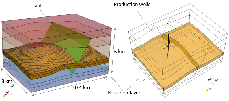
•Various geostatic initialization phases (gravity, tectonic, contact release, constitutive release) •Production simulation •Mechanical contact •Initial spatial grid data and spatial boundary |
|
•Case 1b Reservoir Poro-elasticity defined via Spatial_table |
•Young's modulus - porosity dependent spatial table |
|
•Geostatic initialization stages (gravity and tectonic) via implicit solver •Restart data |
||
•Case 3a HM Coupled (High Perm Fault) •Case 3b HM Coupled (Low Perm Fault)
|
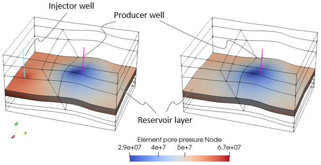
•Coupled HM simulation •Water level •Well element for producer well •High/Low perm contact fluid flow •Initial spatial grid data and spatial boundary |
|
•As Case 3a •Well element for producer and injector wells |
||
•As Case 4 •De-activation of porous flow groups |
||
•As Case 4 •Full implicit solver utilized for coupled hydro-mechanical solution •Node-node contact algorithm |
||
•Case 5 Mapping of Results to Spatial Surface and Output to Plot File |
•Read results plot file and output to new plot file •Mapping of results to imported Spatial surface definition |
|
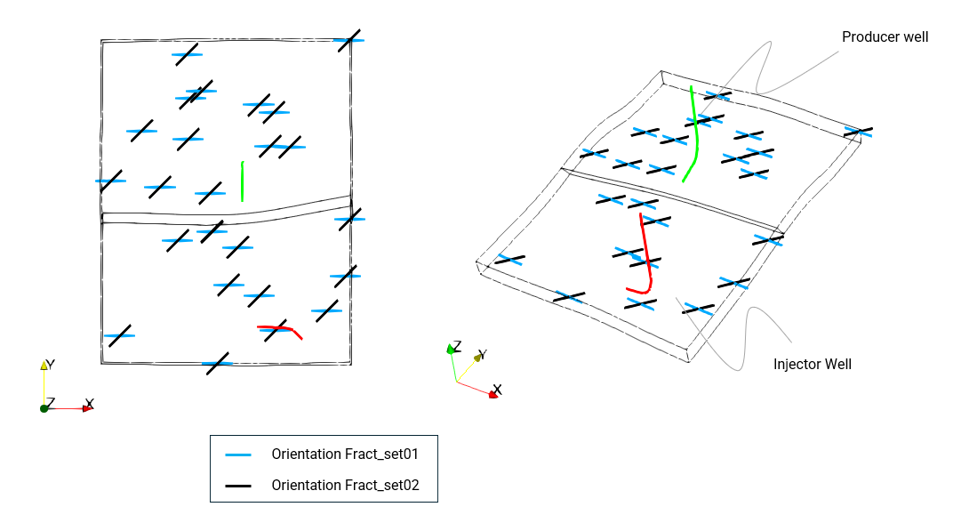
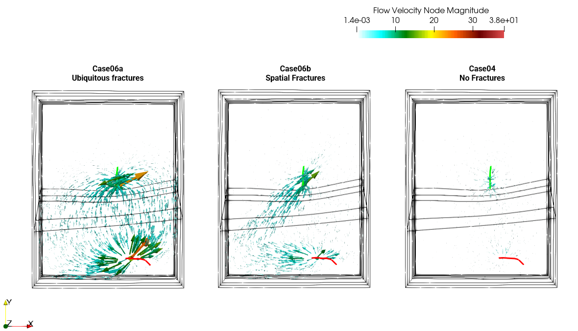
•Case 6 Reservoir with Fractures oCase06a - Ubiquitous fractures with homogeneous properties with fracture spacing of 5m oCase06b - Two corridors of fractures with spatial definition of fracture spacing ranging from 25m to 75m |
•Inclusion of embedded fractures in the reservoir and their influence on pore pressure distribution and flow |
|
Mechanical (3D) |
|
|
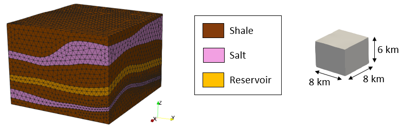
•Case00 Scaling Salt Viscosity
|
•Salt layers modelled via Herschel-Bulkley viscoplastic material •Various time unit updates via salt material constant K |
|
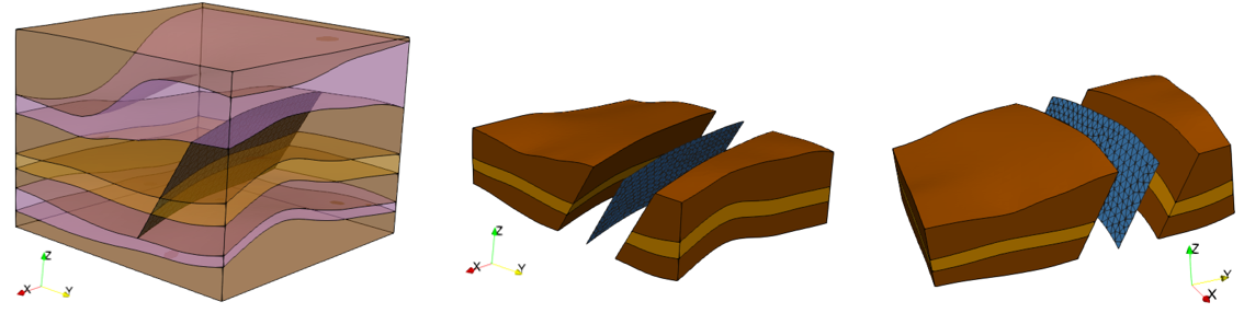
•Case 2 Faulted Case (Not available yet) |
•Faulted model with contact |
|
MEM_003 Boundary Optimisation and Super Element approach within the MEM Workflow |
Mechanical (3D) using ParaGeoInv |
|
•Case 2 Boundary optimisation using the Super Element approach (Currently unavailable) |
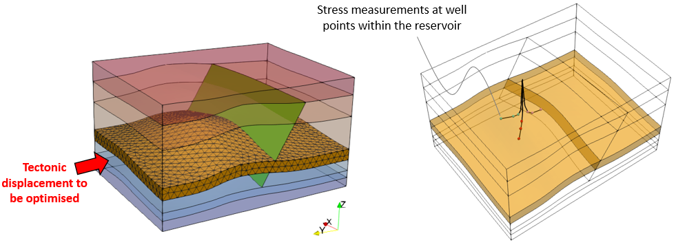
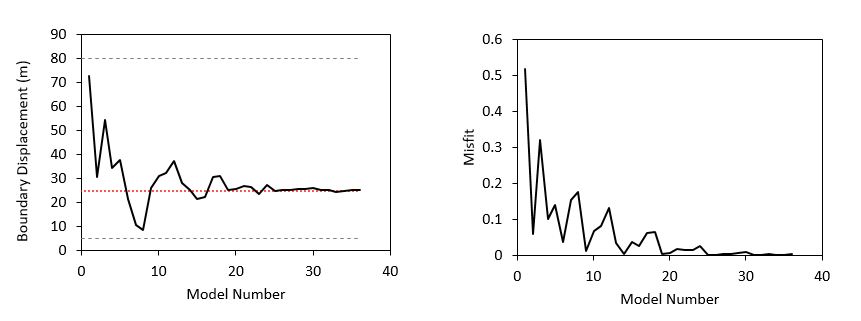
•Inverse analysis for initialisation stages using ParaGeoInv •Usage of Super element |
|
Implicit Solver |
||
Mechanical (3D) |
|
|
•Implicit solver |
|
|
Super Element (Currently unavailable) |
||
SuEl_001 Super Element Workflow |
Mechanical (3D) |
|
•Case 1 Workflow Example oStep 1 Create the Super Element oStep 2 Use the Super Element oStep 2b Use an Reflate the Super Element •Case 2 Usage of Coupled Freedoms |
•Super element workflow •Implicit solver •Coupled freedoms |
|
Geological Modelling Workflow |
||
Mechanical (2D) |
|
|
•Geometry .dxf preparation in CAD •.dxf to ParaGeo geometry .geo workflow •Restoration with decompaction •Forward simulation •Utility to create forward model data from restoration |
|
|
ParaGeo Utility Mechanical & Coupled THM (3D) |
|
|
•Zmap file import and export to Abaqus .inp file utility •Conversion of .inp file to ParaGeo .geo file •Hydrocarbon generation layers •Restoration modelling (geomechanical) •Sedimentation modelling (THM) •Moving water table with time •Directional decompaction •Boundary node extraction from irregular boundaries •Hexahedral mesh model •Basal thermal flux |
|
|
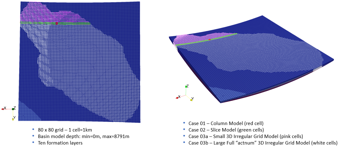
•Case03a 3D Small Irregular Grid Model with 'Ragged' Boundaries |
||
•Case03b 3D Large Irregular Grid Model with 'Ragged' Boundaries |
||
Mechanical & Coupled THM (3D) |
|
|
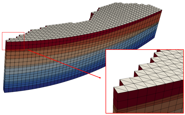
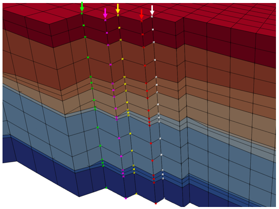
•Membrane elements for bed length preservation •Boundary column nodes with coupled freedoms |
(a) Membrane (triangle) elements on top surface (b) Column of coupled nodes on boundary |
|
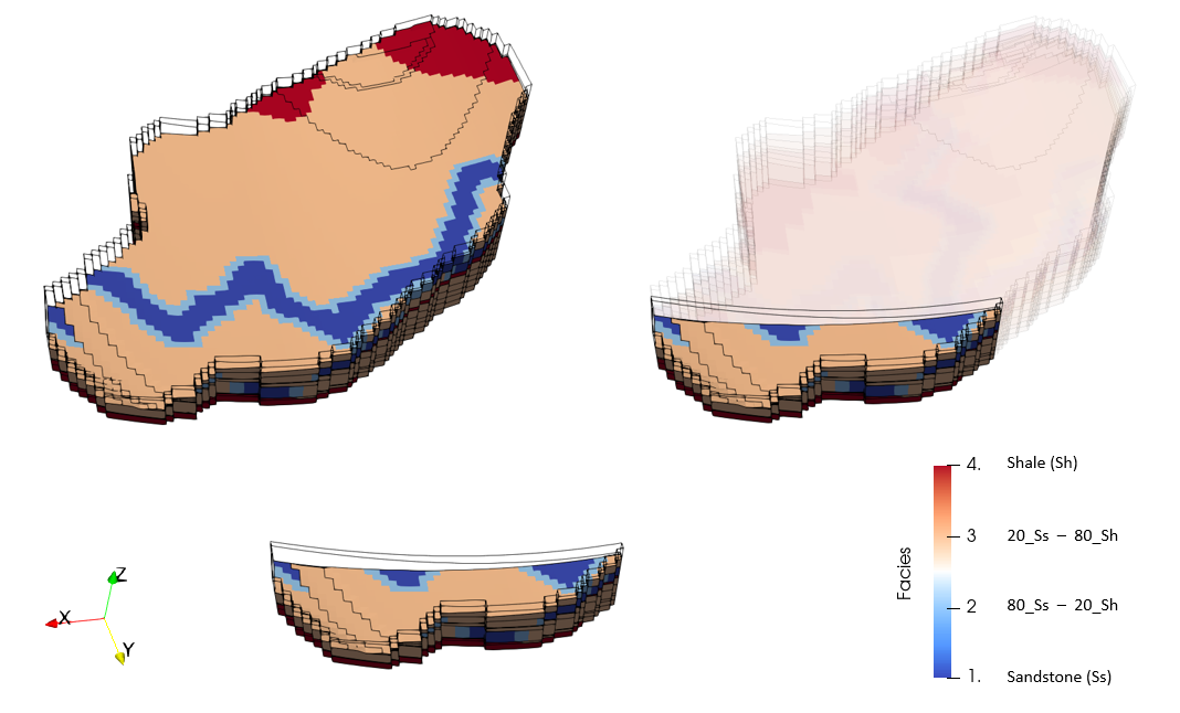
•With spatial distribution of material property facies |
Facies distribution in Formation 08 in tutorial sub-model |
|
•With erosion in restoration & sedimentation |
|
|
•With spatial distribution basal heat flux |
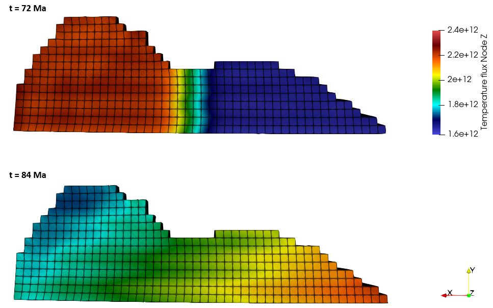
Basal heat flux distribution |
|
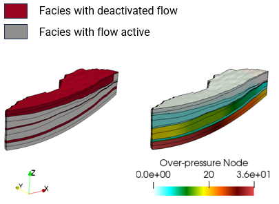
•Case05 Additional functionality for Facies modelling oCase05a Standard reference case oCase05b Facies with deactivated fluid flow oCase05c Facies with permeability multipliers oCase05d1 Facies with advection terms active oCase05d2 Facies with advection terms deactivated |
•Additional functionality for Facies: oDeactivation of fluid flow oPermeability multipliers oDeactivation of advective heat flow |
Large overpressure due to no flow across or along seals |
ParaGeo Utility Mechanical (3D) |
|
|
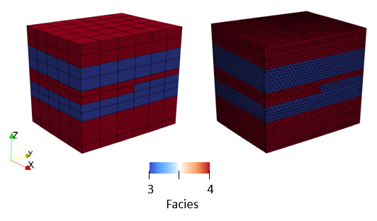
•Zmap file import and export to Abaqus .inp file utility •Conversion of .inp file to ParaGeo .geo file •Hex to TET conversion •Restoration modelling with adaptivity (geomechanical) •Utility to create forward model data from restoration •Sedimentation modelling (geomechanical) •Spatial distribution of facies |
Facies distribution from zmap (left) and after forward modelling (right) |
|
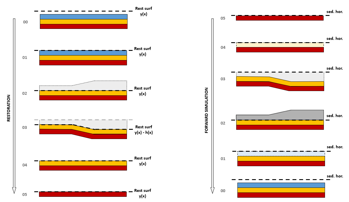
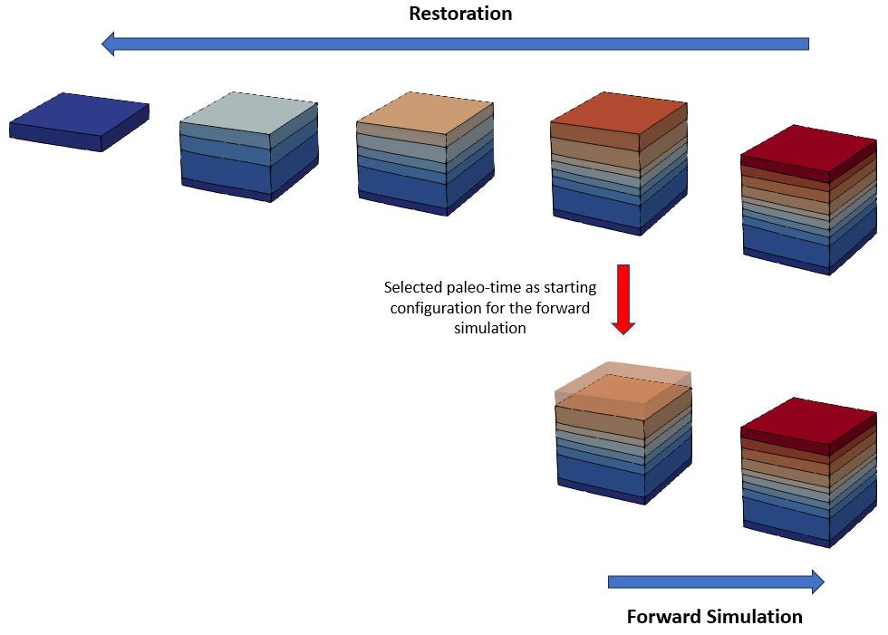
•Case02 Forward simulation from a non-final restoration paleo-time |
•Utility to read plot file results and export a spatial grid •Utility to create forward model data from restoration •Sedimentation modelling (geomechanical) •Spatial distribution of facies |
Schematic of the workflow |
Hydrocarbon Maturation |
||
Coupled THM (2D) |
|
|
|
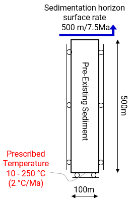
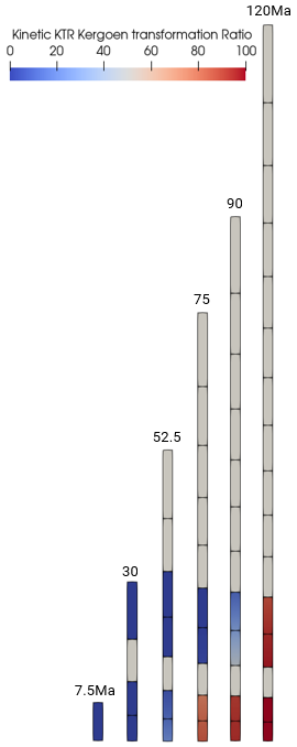
•THM sedimentation •Multi-kerogen sediment layers •Influence of HC kinetics on pore pressure, porosity and strength •Combined use of two damping models for long column |
|
Parameter Definition |
||
Mechanical (2D) |
|
|
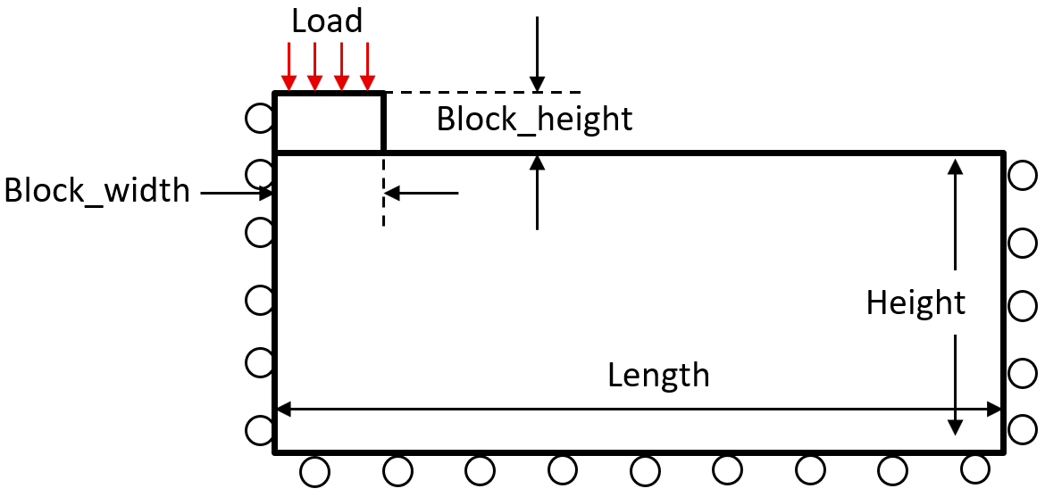
•Parameter definition (various usage)
|
Strip footing model |
|
Wellbore Models |
||
Coupled THM (3D) |
|
|
•Case01 Time-dependent Cement Hardening with Diagenetic Shrinkage |
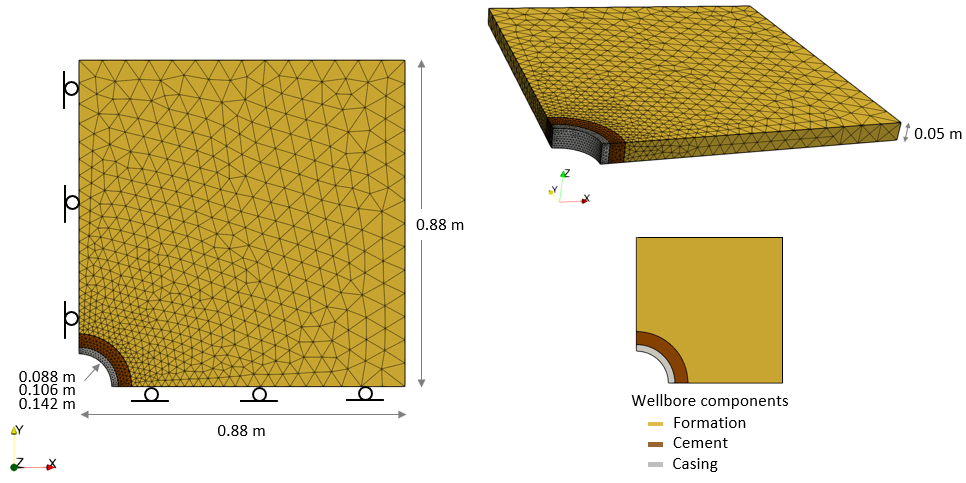
•Coupled THM simulation •Deactivated porous flow in casing and cement •Contact between wellbore components •Time-dependent cement hardening material with increased yield strength •Cement hardening with diagenetic reaction resulting in volume shrinkage •Usage of transient time step growth in solution control |
|
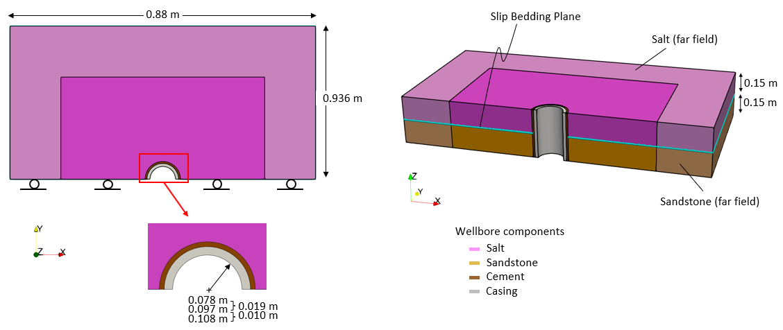
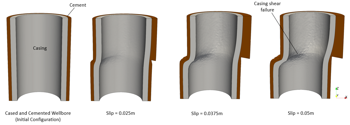
Wellbore_002 Casing Collapse due to Shear at Salt/Sandstone Bedding Plane |
Mechanical (3D) |
|
|
•Contact between salt/sandstone bedding plane •Large bedding plane slip (shear) causing casing collapse •Salt with Herschel-Bulkley viscoplastic material |
|