Case 1a Poroelastic simulation
In the first case for the fractured specimen under depletion-injection conditions a poroelastic material will be considered.
Basic Set Up: Data file description
The initial data file for the project is: Mat_003\Data\Mat_003_Case1a.dat. The basic data includes: 1Units data defining the units of the problem. 2A single Group_data structure for the single element and Group_control_data to define the group as active for geomechanical and fluid flow fields. 3Material properties of the reservoir are defined via the following data structures: a.Material_data defining the porous matrix properties b.Fluid_properties defining the pore fluid c.Fracture_data assigned to the material defining the fracture properties d.Coordinate_system assigned to the fracture defining fracture orientation. 4Support_data defining the displacement constrains. 5Couple_freedoms on the top surface ensuring that the displacement is consistent in the top surface nodes 6Two Global_loads data structures to define the vertical stress load (overburden) and the pore pressure load with their corresponding Time_curve_data structures. 7Load_case_control_data to define the previous loads as active during the simulation. 8Mesh control (Mesh_control) and Structured mesh generation data (Structured_mesh_data) defining a single element. 9Couple_control data defining coupling between geomechanical and fluid flow fields 10Time_scaling_data defining a target optimal time step of 1.0E-4 days. 11History_point data defining the variables that will be output. 12Geostatic_control_data for the two initialization stages. 13Control data (Control_data) for three stages defining (two initialization stages + one for the test simulation): (a) Incremental transient solution algorithm (Type 4), (b) Factor of critical time step = 0.25, (c) Initial time increment (flow step size) of 0.01 days (d) Maximum number of time steps of 200 (coupling steps). (e) Termination times at 1 and 3 days respectively (f)Target number of mechanical steps per flow step of 100. (g) Plot file output every 0.1 days of simulated time, (h) Plot file output at the end of the stage, (i) Screen message output every 10 flow steps, 14Geometry data (nodal_data, Geometry_line, Geometry_surface and Geometry_volume) for definition of the 3D geometry.
|
Results
The result files for the project are in directory: Mat_003\Case1\Results
A simulation of a 10 m specimen with a vertical fracture set has been simulated by applying PVC type boundary conditions (boundary conditions which aim to replicate evolution of pore pressure during reservoir production cycles). As it has been explained above the simulation consisted in 3 stages:
1.Initialization stage 1: Initialization of the model at reservoir initial stress and pore pressure state.
2.Initialization stage 2: Displacement reinitialization and reset of porosity and state variables. During this stage the displacement, porosity loss and any change in state variables that occurred because of the application of the initial conditions during stage 1 is recovered.
3.Reservoir production simulation stage with the following boundary conditions: a.t=1.0 to t=2.0: Pore pressure decreases from 82.5·106 Pa to 55.0·106 Pa. b.t=2.0 to t=2.5: Pore pressure increases from 55.0·106 Pa to 65.0·106 Pa. c.t=2.5 to t=3.0: Pore pressure decreases from 65.0·106 Pa to 50.0·106 Pa.
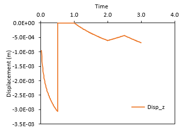
In the figure below the displacement history is shown including the initialization phase. It can be seen that during the first initialization stage (t=0 to t=0.5) a displacement of 3 mm occurred because of the application of initial stresses and pore pressure. It can be seen as well that at the beginning of the second stage (t=0.5 to t=1.0) the displacement is reset to 0 thanks to the displacement reinitialisation specified in Geostatic_control_data. This is useful to output from t=1.0 onwards the absolute displacement occurring because of the reservoir production cycle. Note that the following figures will omit the initialisation history and the focus will only be in the PVC test simulation.
It can be seen that from t=1.0 to t=2.0 there is some negative displacement resulting from the drop in pore pressure which in turn resulted in increase in stresses. This is followed by elastic recovery of some displacements from t=2.0 to t=2.5 due to the pore pressure increase and subsequently there is more elastic displacement beyond the previous maximum displacement due to the drop of pressure to a minimum value (and hence maximum stresses).
Displacements as a function of time (including initialisation)
In the figure below the evolution of stresses and pore pressure is shown. It can be seen that:
1.As expected the effective mean stress and deviatoric stress (Vonmises) show a negative correlation trend with pore pressure. 2.The stress path in the p'-q space (figure on the right) shows an elastic path in which the unloading path coincides with the loading and reloading path. 3.The increment in stress in Y direction is lower than the increment in stress in the X direction. This is due to the influence of the fractures which are perpendicular to the Y axis and therefore they will accommodate part of the stress change by fracture closure.
Evolution of stresses and pore pressure
Different compressibilities for the reservoir can be calculated. Those are: •Pore volume compressibility (neglecting temperature effects), which stands for the porosity change due to changes in pore pressure (D(phi)/D(pf) in the graph):
•Compressibility as a function of the change in the effective mean stress (D(phi)/D(peff) in the graph):
•Elastic compressibility:
Where:
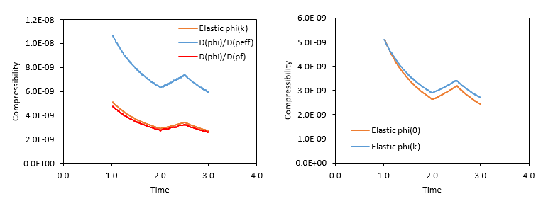
In the left figure below the evolution of the different calculated compressibilities can be seen. It can be noted that: 1.There is a small difference between the elastic compressibility and the pore volume compressibility as expected given the poroelastic assumptions in the material. 2.There is a significant difference between the pore volume compressibility and the compressibility that accounts for the change in the effective mean stress. This is due to the fact that even though the total vertical stress is constant (as overburden weight is constant) the total horizontal stress varies. Therefore, even for the present case in which Biot's constant is 1.0, the change in pore pressure does not coincide whit the change in the effective mean stress.
In the figure on the right hand side there is compared the evolution of the elastic compressibility as defined in ParaGeo (phi(k) in the figure) with a definition of the elastic compressibility found in the literature (e.g. Dean et al. (2006), phi(0) in the plot) which is calculated as:
Note that the difference relative to the ParaGeo definition of the elastic compressibility is that it is evaluated considering the initial reference porosity for the reservoir (
Evolution of compressibilities
In the figure below evolution of matrix porosity, permeability and stiffness are plotted. It can be observed that: 1.Porosity follows a positive correlation trend with pore pressure; i.e. when pore pressure decreases there is a porosity loss due to the increase in stress. 2.Matrix porosity loss is rather small (less that 2 porosity units) for a significant change in stresses (e.g. more than 107 Pa of difference in the effective mean stress). This is expected given the poroelastic assumptions for the material. 3.As expected matrix permeability shows a positive correlation with porosity as matrix permeability is calculated as a function of porosity according to the data specified in Material_data. 4.Young's modulus show a positive correlation with effective mean stress. Note that for the poroelastic model chosen to simulate the constitutive response of the material the bulk modulus (and hence Young's modulus) is dependent on the effective mean stress so that the higher the effective mean stress, the higher the Young's modulus.
Evolution of some matrix properties with time
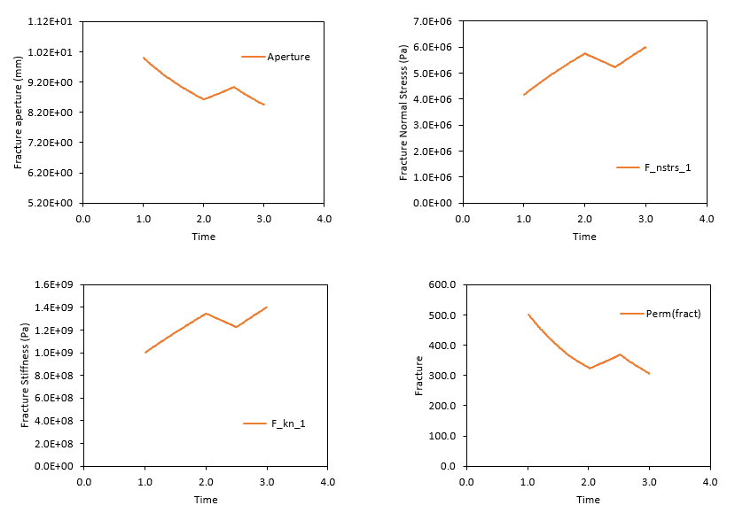
Below the evolution of the fracture state variables is shown. It is recalled that the fracture constitutive response should be non-linear elastic as specified in Fracture_data. It can be seen that: 1.Fracture aperture shows a positive correlation with pore pressure. This is because when pore pressure decreases the stress in Y direction (which is perpendicular to the fracture planes) increases leading to some fracture displacement. 2.As expected fracture normal stress shows a negative correlation with pore pressure. 3.As expected fracture stiffness shows a negative correlation with fracture aperture so that the more closed a fracture is the stiffer it becomes. This is agreement with the higher contact between both sides of the fracture plane. 4.Fracture permeability shows a positive correlation with fracture aperture in agreement with the input fracture permeability law in Fracture_data.
Evolution of fracture properties with time
Below there are the matrix porosity and permeability as well as fracture permeability plotted as a function of pore pressure. As explained above all these properties show a positive correlation with pore pressure due to the negative correlation between pore pressure and stresses.
Matrix and fracture properties as a function of pore pressure
|
References
Dean, R.H., Gai,X., Stone, C.M. and Minkoff, S.E. (2006). A comparison of techniques for coupling porous flow and geomechanics. SPE Journal, 11(1), 132–140.
|


