HM_004 Uniaxial Sedimentation using Layer Deposition

Contents
This example extends the uniaxial consolidation example HM_001 by considering overpressure build up and dissipation during the sedimentation of a 1000m column represented by layer sedimentation. The layers are deposited as layers of discrete thickness using a general layer sedimentation algorithm. Note that this algorithm, although not required for this example, allows general intersection of the new sediment layer with existing sediment.
Specific issues considered are:
1Deposition using layer sedimentation for coupled problems.
The example documentation assumes that the user has undertaken the following examples beforehand:
1Mech_002 Uniaxial Burial of a 2000m of Sediment. This describes the layer sedimentation algorithm.
2HM_001 Introduction to Hydro-Mechanical Analysis - Uniaxial Consolidation.
3HM_002 Uniaxial Sedimentation using Pre-Existing Sediment.
The objective is to simulate the sedimentation and consolidation of 1000m of sediment over a period of 1.0 Ma. Only 20m of pre-existing sediment is represented and sedimentation is represented by the layer sedimentation algorithm.
The model is analysed in uniaxial strain conditions; i.e. the vertical sides of the model are constrained in the horizontal direction, and the base of the model is constrained in the vertical direction. Gravity is the only load and the top surface of the model is prescribed zero pore pressure (pf); i.e. free drainage, resulting in a gradual dissipation of pore pressure in the model.
A two stage analysis is performed: In stage1, the gravity load for the pre-existing sediment is applied over 0.1 Ma followed in stage 2 by sedimentation of the column between 0.1 and 1.1 Ma. An unstructured mesh of triangular (TPM3V) elements is used with a target element size of 20m. Adaptive remeshing is required for stage 2 due to the sedimentation process. Remeshing is triggered at a distortion of 15% with the objective of maintaining the element size at 20m.
Material Properties The material parameters corresponding to "HM_002_elastic" material are chosen to match the parameters assumed in the simulations presented by Wangen (2010, p.403). The primary mechanical properties for this material are:
The additional material parameters related to the porous flow field are:
Notes 1The simulation uses isotropic permeability. In general, however, soils exhibit transverse isotropic flow with the horizontal permeability often between 5 to 100 times larger than the vertical permeability. In this case orthotropic permeability may be defined via Permeability_x, Permeability_y and Permeability_z. Furthermore, permeability is dependent on the current porosity, so that in applications where significant compaction is used permeability is defined as a function of porosity. This may be either isotropic via Permeability_vs_porosity or orthotropic via Permeability_x_vs_porosity, Permeability_y_vs_porosity and Permeability_z_vs_porosity. 2The Biot constant (Biot_constant) defines the contribution of the pore pressure to the total stress via the effective stress relationship
The Biot constant may either be user defined (as in this case) or may be computed automatically via the relationship
3The material is specified as fully saturated ( Fluid_saturation = 1.0). 4The material is saturated with fluid name "Water".
Fluid Properties The properties of the pore fluid must be specified. The principal parameters are:
|
The initial data file for the project is: HM_002\Case1\Data\hm_002_Case1.dat. The basic data includes:
1Units defining stress in "MPa", length in "m", time in "Ma" and temperature in "Celsius". 2Geometry_set data defining model boundaries and domain. 3Mesh control (Mesh_control_data) and unstructured mesh generation data (Unstructured_mesh_data defining a uniform mesh with size of 20m. 4A single group which is assigned the "hm_002_elastic" material properties defined using Group_data and Group_control_data data structures. The Porous_flow_type = 4 i.e. a coupled geomechanical/porous flow. 5Material properties (Material_data) for "hm_002_elastic". 6Fluid properties (Fluid_properties) for water. 7Stratigraphy_definition and Stratigraphy_horizon to define the pre-existing stratigraphy unit and top surface. Stratigraphy_surface_load to define a prescribed pore pressure condition (Pore_pressure_flag set to 1) on the top surface. 8Sedimentation_parameters, Sedimentation_horizon and Sedimentation_data defining sedimentation data for the new layers. 9Geostatic_data defining initial pore pressure of 0 MPa for the pre-existing sediment. 10Support_data defining geomechanical fixity constraints: base fixed vertically and sides fixed horizontally. 11Damping_global_data defining the use of combined damping models (percentage damping of 2%, i.e. 0.02 and bulk viscosity damping with constant of 0.5) to aid the numerical stability of the column model. 12History data: (a) Global history (History_global) data to output every 0.01 Ma the energies (dynamic response) for the complete domain. (b) Point history (History_point) data to output every 0.01 Ma the stresses, pore pressures and porosities at a point in the middle of the pre-existing layer. 13Solution control data via coupling control data (Couple_control_data) and geomechanical/porous flow control data (Porous_flow_control_data and Control_data) (see later).
|
The stratigraphy associated with the initial pre-existing sediment must be defined when the layer sedimentation procedure is used. This requires 1Defining the existing stratigraphy layer depositional order and the group associated with each layer (via Stratigraphy_definition). 2Defining the topology of the top surface horizon for each stratigraphy layer (via Stratigraphy_horizon).
Stratigraphy_definition The stratigraphy order is specified in order starting from the deepest sediment layer. Each stratigraphy layer must comprise a single group (see Group_data). It is recommended that, for each layer, the stratigraphy unit name, stratigraphy horizon name and group name are identical. This greatly simplifies data definition and result interrogation, especially when the number of stratigraphy layers becomes large. If this convention is adopted, ParaGeo will internally identify the required associations between unit, horizons and groups, so that only the unit order is required to be defined in the Stratigraphy_definition data structure.
Stratigraphy_horizon The stratigraphy horizon defines the top surface of each pre-existing stratigraphy unit. It is defined by a set of geometry lines in 2-D or a set of geometry surfaces in 3-D. A Stratigraphy_horizon data structure must be defined for each stratigraphy unit.
|
Layer sedimentation is defined using three data structures: 1Sedimentation_data which defines the control data for deposition of a single layer; e.g. unit name, material, sedimentation type, etc. 2Sedimentation_parameters which defines the data that is common to the deposition of all layers. 3Sedimentation_horizon which defines the target topology for the stratigraphy horizon of the new layer.
Note that a Stratigraphy_horizon is an existing horizon defined by geometry entities (lines 2-D, surfaces 3-D) that form part of the model, whereas a Sedimentation_horizon is a faceted surface that is not connected with the model. During layer sedimentation new geometry entities are created to define the new layer, and the Stratigraphy_horizon for the new layer is formed using a combination of these new geometry entities and pre-existing geometry (if required).
Sedimentation_data Sedimentation_data is the primary data structure for definition of sedimentation of a new stratigraphy unit. One data structure is required for each new layer and the sedimentation process is associated with a single analysis stage. Consequently in the current problem, where ten additional layers are deposited on top of the pre-existing layer, the sedimentation process consists of 11 analysis stages. Sedimentation_parameters is used to specify data that is common to all sedimentation steps/stages. Consequently the only data required to add a new layer in Sedimentation_data is the unit name.
Sedimentation_Parameters Sedimentation_parameters is used to define data that is common to all sedimentation steps and these parameters will be used for each sedimentation step by default. The value of any parameter can be replaced for a particular sedimentation step by specifying the same parameter with a different value in the Sedimentation_data data structure for that step. The principal data includes: 1The sedimentation horizon name (Sediment_horizon_name); i.e. the Sedimentation_horizon to be used in defining the top surface of the new layer. 2The name of the material properties to be used for the new material (Material_name). 3The duration (Duration) of the initialisation of gravity loading for the new layer.
Note that by default, the Sedimentation_type is "Absolute" where the Sedimentation_horizon defines the top surface of the new layer. Two alternative sedimentation types are available: 1"Relative" - where a sedimentation horizon defines the topology of the new top surface but its location is defined via a layer thickness (Reference_thickness) and reference location (Reference_location). 2"Drape" - Where a uniform thickness of material is added across the complete model.
Sedimentation_Horizon The Sedimentation_horizon data structure defines the topology of a top surface horizon for sedimentation of a new stratigraphy layer. The horizon is defined as a faceted surface; i.e. 2-noded facets in 2-D, 3-noded facets in 3-D. The node numbering and coordinates defining the faceted surface are defined in the data structure and do not form part of the nodes in the mesh. The horizon may be defined as either stationary or moving; e.g. increasing in elevation or prograding, via a displacement component magnitude and a time curve. A sedimentation horizon may be used to define more than one layer; e.g. a prograding horizon is often used to define sedimentation of all layers. Alternatively multiple sedimentation horizons may be specified and used for the sedimentation of individual layers.
|
Analytical equations for the development of overpressure in in a basin at constant sedimentation rate were developed by Gibson (1958) and further discussed in Gibson (1967) and Wangen (2010) amongst others. The solution assumes a shallow basin where the porosity reduction is negligible; i.e. the geometrical impact of compaction may be neglected. The key assumption of the model is that Porosity (φ) is a linear function of the vertical effective stress (σ'v); i.e.
Substitution in the mass conservation equation and solution for the special case of constant sedimentation rate and zero surface pore pressure then gives
Note that rearrangement of the expression for porosity gives
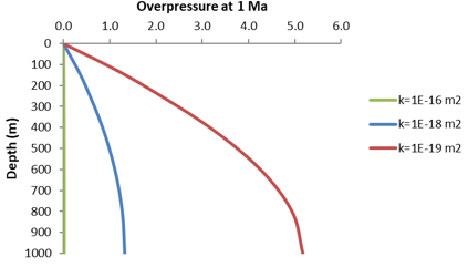
Wangen (2010, p.403) provides overpressure predictions for a particular set of material parameters comprising;
A solution, obtained by very approximate integration using a multi-point trapezoidal rule, is provided in Excel worksheet HM_004\Results\00_hm_004.xlsx "Analytical" worksheet.
Overpressure at 1 Ma for three Different Permeability Values
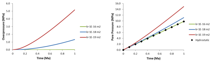
Overpressure at the Base of the Column vs. Time for three Different Permeability Values
References Gibson, R. E. 1958. The progress of consolidation in a clay layer increasing in thickness with time. Géotechnique, 8, 171–182. Gibson, R. E., England, G. L. & Hussey, M. J. L. 1967. The theory of one-dimensional consolidation of saturated clays. Géotechnique, 17, 261-273. Wangen, M. 2010. Physical Principles of Sedimentary Basin Analysis, Cambridge University Press.
|
The result files for the project are in directory: HM_004\Results. The high definition history files are displayed graphically in the excel file HM_004\00_hm_004.xlsx.
Two cases are considered: •Case 1 - where the permeability (k) = 1.0E-18 m2. •Case 2 - where the permeability (k) = 1.0E-19 m2.
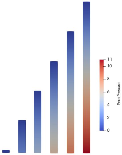
Case 1 Permeability (k) = 1.0E-18 m2 The evolution of pore pressure as a function of column height is shown in the figure below.
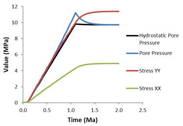
The evolution of pore pressure as a function of time exhibits a marked change at time 1.1Ma corresponding to the end of sedimentation. The overpressure is completely dissipated by the end of the simulation at t = 2Ma. The vertical and horizontal effective stresses increase during this period to compensate for the reduction in pore pressure.
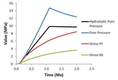
Pore Pressure and Stress Evolution at the Base of the Column as a Function of Time
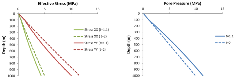
Effective Vertical Stress and Pore Pressure with Depth at t = 1.1Ma and t = 2Ma
Case 2 Permeability (k) = 1.0E-19 m2 As expected the evolution of pore pressure as a function of time exhibits significantly higher pore pressure than Case 1 where (k) = 1.0E-18 m2.
Pore Pressure and Stress Evolution at the Base of the Column as a Function of Time
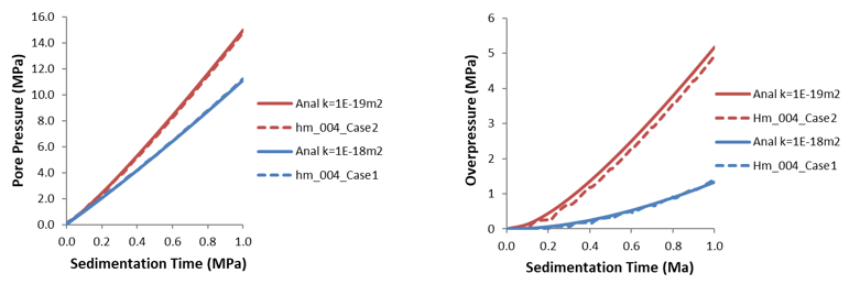
Comparison with Analytical Solution Comparison of the analytical solution with the predicted pore pressures obtained by layer sedimentation shows very good correlation between the two solutions for both perm cases. However, the predicted overpressure for the lower perm case k=1E-19m2 could be improved with an "undrained" solution algorithm instead of a "fixed stress" algorithm.
Comparison of Pore Pressure Evolution at the Base of the Column as a Function of Time for HM_003_Case1 and HM_004_Case1
|