Case02 Boundary Optimisation Using the Super Element


The present case is identical to Case01 except that the super element approach is used in the optimisation procedure. Hence it is recommended to be familiar with Case01 and have undertaken the SuEl_001 tutorial example beforehand.


When using the super element in the optimization procedure the set up of the .inp file and folder structure is mostly identical with the only differences being:

1.The super element must be created before running the optimisation procedure

2.The template data file must include Super_element_control data structure set to use the super element


The data for the present case is provided in MEM_003\Case02\Data. For the present case the folder structure includes an additional folder in MEM_003 \Case02\Data\Create SE where the super element is created.


Super Element Creation


The creation of the super element for usage in the optimisation procedure follows a two step process that requires to run the files MEM_003_Case02_Create.dat and then MEM_003_Case02_Use.dat


MEM_003_Case02_Create.dat


The MEM_003_Case01_Create.dat file is identical to the first stage of the template data file except that it includes a Super_element_control data structure set to Create the super element (the template must be set to Use the super element). Note that in the present case Couple_freedoms will be used to optimise the super element file size.


Super Element-related data


Data File


* Super_element_control

! ---------------------------------

 Field                      "Gmech"

 Solution_type             "Create"

 File_name         "MEM_003_Case02"

 Retained_couple_freedoms  IDM=1

   1

 Retained_history_sets  IDM=3

  "points_prod_well_1"

  "points_prod_well_2"

  "points_prod_well_3"


* Couple_freedoms  NUM=1

! ---------------------------------

 Geomechanical_codes IDM=3

   0 1 0

 Geometry_sets   IDM=1

   "North"        


* History_point  NUM=1

! ---------------------------

 Name              "points_prod_well_1"

 Output_frequency_increment          -1  

 Point_labels   IDM=3

 "W1_P1"        

 "W1_P2"

 "W1_P3"

 Point_coordinates  IDM=3  JDM=3

 /W1_P1/  4150   6750  3200

 /W1_P2/  3900   7000  3000

 /W1_P3/  3500   7400  2800

 Stresses  IDM=3

   "Strs_xx"  "Strs_yy"  "Strs_zz"


* History_point  NUM=2

! ---------------------------

(...)


* History_point  NUM=3

! ---------------------------

(...)


1.Super_element_control is set with data to Create the super element. An optimal choice of the retained components into the super element has been made for the present case. This comprises:


i.Couple_freedoms data structure number 1 which consists of a single node representing the "North" boundary ( see SuEl_001 Case02 for more information on usage of couple freedoms for the super element).


ii.The history point sets. This will retain the element that contain each of the points defined in the point set.


2.The retained Couple_freedoms and History_point data structures are defined.


Note on Fixities during the Super Element Create Step


Data File


* Support_data

! ----------------------------------------

 Displacement_codes  IDM=3   JDM=4

  /Set1/  1  0  0

  /Set2/  0  1  0

  /Set3/  0  0  1

  /Set4/  1  1  1

 Displacement_code_geom_set  IDM=4

   "East"

   "West"

   "South"

   "Base"

 Displacement_code_geom_ass  IDM=4

   1  1  2  3


1.It should be noted that the retained boundaries and/or coupled freedoms should not be applied fixities in Support_data during the super element create step.


2.In this case "North" is not included in Support_data as the coupled freedoms for North boundary are retained.


After running MEM_003_Case02_Create.dat the file MEM_003_Case2.suelmat will be output. Then in the next step of super element preparation this file will be updated.


MEM_003_Case02_Use.dat


The objective of the present step in the preparation process of the super element is to run a single simulation using the super element in order to update the .suelmat file and obtain the .neinods file as required for using the super element within the optimisation context.


The MEM_003_Case02_Use.data file is identical to the template data file (including the two stages) except that the Parameterised_boundary is manually populated with data.


Super_element_control


Data File


* Super_element_control

! ---------------------------------

 Field                      "Gmech"

 Solution_type                "Use"

 File_name         "MEM_003_Case02"

 Solver_optimisation_flag         1


1.Super_element_control data is set to Use the previously created super element.


2.Solver_optimisation_flag = 1 is specified. This is a special flag to make the inversion analysis more efficient as some data required for the analysis will be written to the super element only during this step rather than being calculated each simulation.


3.Note that Couple_freedoms must not be specified in the "Use" step because a single node representing the "North" boundary has already being retained during the "Create" step (as specified in Reatin_couple_freedoms during the "Create" step)


Parameterised_boundary


The Parameterised_boundary data structure is defined in the second simulation stage (after the first Control_data data structure) with arbitrary data manually populated to run a single simulation.


Data File


* Parameterised_boundary  NUM=1

! ----------------------------------------

Geometry_set             "North"

 Value  IDM=1

   5.0


* Spatial_boundary  NUM=2

! ----------------------------------------

 Name                  "Para_bound"

 Boundary_type       "Spatial_grid"

 Value_type              "Relative"

 Relative_time_curve              1

 Spatial_grids   IDM=1

   "North"

 Prescribed_components IDM=1 JDM=1

   2


1.Arbitrary displacement is populated into the Parameterised_boundary in order to enable to run a single simulation.


2.Note that usage of Parameterised_boundary requires definition of an associated Spatial_boundary (internally the code creates a Spatial_grid for the boundary nodes with the parametrised displacements which are applied via the Spatial_boundary)


Support_data in Use Step


Data File


* Support_data

! ----------------------------------------

 Displacement_codes  IDM=3   JDM=4

  /Set1/  1  0  0

  /Set2/  0  1  0

  /Set3/  0  0  1

  /Set4/  1  1  1

 Displacement_code_geom_set  IDM=5

   "East"

   "West"

   "North"

   "South"

   "Base"

 Displacement_code_geom_ass  IDM=5

   1  1  2  2  3


1.In the "Use" step of the Super Element preparation "North" must be defined in Support_data


After running the file MEM_003_Case02_Use.dat the file MEM_003_Case02.suelmat is updated and the file MEM_003_Case02.neinods is output. Those files will be required to run the optimisation procedure.


Template: Data File Description


The template data file MEM_003_Case02.dat file is identical to Case01 template data file except that it includes Super_element_control data set to Use the super element. In fact the data file is identical to the MEM_003_Case02_Use.dat file in MEM_003\Case02\Data\Create_SE but with the difference that the Parameterised_boundary data is left in blank (as the data will be populated with different displacement values for each model generated by ParaGeoInv).


Super Element Data


Data File


* Super_element_control

! ---------------------------------

 Field                      "Gmech"

 Solution_type                "Use"

 File_name         "MEM_003_Case02"

 Solver_optimisation_flag         1


1.Super_element_control is set with data to "Use" the super element.


2.Solver_optimisation_flag = 1 also needs to be specified to the template data file.


Parameterised_boundary


The Parameterised_boundary data structure is defined in blank. The data defining the displacement magnitude will be populated by ParaGeoInv during the inversion analysis.


Data File


* Parameterised_boundary  NUM=1

! ----------------------------------------

! This data will be populated by ParaGeoInv


* Spatial_boundary  NUM=2

! ----------------------------------------

 Name                  "Para_bound"

 Boundary_type       "Spatial_grid"

 Value_type              "Relative"

 Relative_time_curve              1

 Spatial_grids   IDM=1

   "North"

 Prescribed_components IDM=1 JDM=1

   2


1.Arbitrary displacement is populated into the Parameterised_boundary in order to enable to run a single simulation.


2.Note that usage of Parameterised_boundary requires definition of an associated Spatial_boundary (internally the code creates a Spatial_grid for the boundary nodes with the parametrised displacements which are applied via the Spatial_boundary)


Results


The results for the project are in MEM_003\Case02\Results. In MEM_003\Case02\Results\Test there are results for the file named MEM_003_Case02_186Reflate.dat which is a case manually run with plot file output and reflate results from the optimal model.


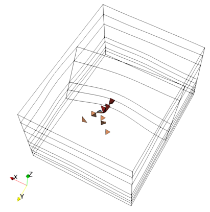
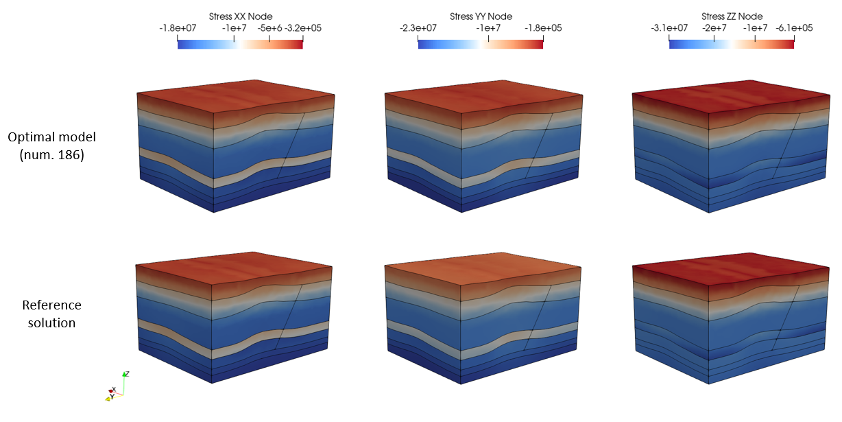
For the present case the iterative algorithm has converged to a value of 24.1 m for the displacement applied to the North boundary although it has not satisfied the convergence criteria imposed, finishing with a Misfit value of 0.1901E-01 (c.a. 2%). Note that the displacement derived from the inverse analysis (24.1 m) has a 3.6% of error relative to the one used to generate the target solution (25.0 m). Nonetheless in the figures below it can be seen that the stress distributions are very similar to the target solution. Also below is provided a figure that shows the retained elements (from the retained history point sets). Note that such figure may be obtained from the plot file from the "Use" stage (as opposed to the "Reflate") by applying a Threshold filter based on a stress element variable and set the maximum stress to a non-zero (negative) value.


MEM_003_Case02_01

Retained elements (from the retained history point sets).


MEM_003_Case02_02

Comparison of stress distributions for the optimal model from the present case and the reference solution.


Standard Simulation vs Super Element Approach


The present case has shown how to use the Super Element (SE) approach within the boundary optimization MEM workflow. The SE is advantageous in that it helps to save computational times when numerous simulations of the same model setup are needed to be performed. For the present case however it runs relatively quickly even using the standard simulation as the model has relatively small number of nodes and elements (9279 and 46488 respectively). Thus with the aim of demonstrating the benefits of the SE approach in terms of CPU time savings a finer mesh version of the current model has been run (both standard simulation and with the super element approach).


The finer mesh version of the model has c.a. 898,000 nodes and c.a. 5,365,000 elements. Although many MEMs may have meshes with many more elements and nodes than that (of the order of 1 order of magnitude more elements) this setup is enough to demonstrate CPU time savings. In addition it has to be noted that when using the implicit solver RAM memory may be a technical-limiting factor as it is easy to run out of memory for models with a large number of elements. Thus it is generally recommended to perform the optimisation procedure with a coarser mesh version of the model of interest as the differences of the optimised displacement are expected to be rather small compared to the original model. The CPU times associated to the simulations are provided in the table below.


Standard Simulation

SE approach

SE Create

---

6929.0 sec

Simulation

3176.0 sec

12.38 sec

CPU times obtained from different runs with and without the super element approach


As can be derived from the table above the SE approach in such case provides a clear benefit in CPU time saving with a speed up factor on the simulation time of 256. As can be seen the CPU time spent on creating the Super Element is similar to the time spent on two standard simulations. Hence the benefit of applying the SE approach is gained even after the first sample of models run during the optimisation procedure (as more than two models per sample are expected). To have an idea on the time savings lets consider an inversion analysis that would require 20 samples of 6 models each to converge to an optimised displacement. The standard approach will accumulate a total CPU time of 4.4 days whereas the Super Element approach would only require 2.3 hours.