Case01 Boundary Optimisation

Contents

In order to perform the inverse analysis a folder structure with a template datafile (that will be used to generate all the models data files), the data used as target results need to be defined in addition to the main data file (.inp) defining the inverse analysis data. The starting folder structure with the data required is provided in MEM_003 \Case01\Data and is as follows:

•Target: folder containing the target results file(s) to be used for optimisation of the boundary condition.

▪MEM_003_Ref_001.hdh

▪MEM_003_Ref_002.hdh

▪MEM_003_Ref_003.hdh

•Template: folder containing the template data file(s) that will be used to define all models simulation data files.

▪MEM_003_Case01.contact

▪MEM_003_Case01.dat

▪MEM_003_Case01.geo

▪MEM_003_Case01.geometry

▪MEM_003_Case01.mat

▪MEM_003_Case01_Porosity.spat

▪MEM_003_Case01_PP_Initial.spat

•Test: folder to which the simulations will be run to.

•MEM_003_Case01.inp: Data defining the inverse analysis.

For the present tutorial example the user is assumed to be familiar with ParaGeo and only the data relevant to the inverse analysis and boundary optimisation will be discussed in detail.

MEM_003_Case01.inp file

The MEM_003_Case01.inp file is the main file in which the data associated to the inverse modelling / optimisation procedure is defined. The data structures and all their corresponding keywords defined within this file are described in the GeoInv Data Structures manual section.

Application_data

The Application_data data structure is used to define main controls associated to the code and algorithm used for the inverse modelling procedure.

Data File

* Application_data

! --------------------------------------

Application "Parageo"

Inversion_algorithm "NAInverse"

Executable_name "Parageo"

Executable_directory "C:\parageo\x64"

Experiment "Boundary"

1.The Application (code) used to run the inverse analysis is set to "Parageo". Note that ParaGeoInv has been designed to be flexible and allow usage of different geomechanical codes to run the simulations performed during the inverse analysis.

2.The Inversion_algorithm is set to "NAInverse" which corresponds to the Nearest Neighbour Algorithm (only option currently available).

3.Executable_name defines the name of the .exe file used to run the simulations.

4.Executable_directory may be defined in order to specify a directory for the .exe to use in the analysis. If not set the executable in the PARAGEOHOME environment variable path will be used.

5.Experiment is set to "Boundary" defining that the optimisation procedure is going to be run for a boundary condition.

Boundary_opt_parameters

The Boundary_opt_parameters is the data structure used to define the type of boundary condition to be optimised, the initial value for the boundary condition and the allowed range of values for the boundary condition in the models to be generated by the optimisation procedure. This data is going to be used to populate the blank Parameterised_boundary data structure defined within the template data file.

Data File

* Boundary_opt_parameters NUM=1

! ----------------------------------------

Name "North"

Geometry_set "North"

Type IDM= 1

Value IDM=1

0.0

Minimum_value IDM=1

Maximum_value IDM=1

1.A name for the Boundary_opt_parameters data structure is defined.

2.The Geometry_set for the boundary with the applied displacement to be optimised is defined. In the present case the boundary to be optimised is named "North".

3.Type defines whether the Parameterised_boundary associated with the present Boundary_opt_parameters should have a fixed displacement value (Type = 1) or a variable value to be optimised (Type = 0) during the optimisation procedure. This is designed to enable fixing values for some parameters without requiring to change the template data file when a multi-parameter optimisation procedure is undertaken.

4.Value allows to define the displacement value when the Type is set to 1 (fixed value). For the present case (Type = 0) it is therefore not used.

5.The minimum and maximum displacement values allowed for the current boundary to be optimised are specified via the Minimum_value and Maximum_value keywords respectively. Hence all the models that will be generated during the optimisation procedure will be populated with displacement values within the specified range. It should be noted that the values refer to normal displacements and are positive for displacements towards the model (compression) and negative for displacements pointing outwards (extension).

NA_options

The NA_options data structure is used to set the options for the Nearest Neighbour Algorithm.

Data File

* NA_options

! --------------------------------------

Algorithm "Auto"

Convergence_tolerance 1.000E-03

Maximum_num_samples 30

Num_models_in_initial_sample 6

Num_models_in_sample 6

Num_models_in_resample 4

Model_delete_option "KeepBest"

Number_models_output 5

Model_clean_option "KeepSpec"

Model_results_keep IDM=1

"History"

1.Algorithm is set to "Auto" which means that the algorithm will automatically stop the iterations/samples once convergence is reached.

2.Convergence_tolerance defines the acceptable error / misfit value for the target solution.

3.Maximum_num_samples defines the maximum number of samples / iterations run in the current optimisation procedure. Thus the optimisation procedure will terminate if either convergence is reached or if the maximum number of samples / iterations has been run before achieving convergence.

4.Num_models_in_initial_sample defines the number of different models (with different boundary displacement values) generated in the first sample.

5.Num_models_in_sample defines the number of different models (with different boundary displacement values) generated in each new sample / iteration. Note that this must be equal or lower than the Num_models_in_initial_sample.

6.Num_models_in_resample defines the number of models from the current sample whose results will be taken into account to generate models for each new sample. Thus in the present case after running a sample of 6 models, the best 4 models (the ones with lower misfit values) will be used to narrow the range for boundary displacement values and generate a new sample of 6 models.

7.Model_delete_option is set to "KeepBest" and Number_models_output is set to 5 so that only the 5 best models (the ones with lower misfit values) are temporarily kept after each new resample (the other models are deleted). Hence at the end of the optimisation procedure the 5 best models will be kept.

8.Model_clean_option defines what data to preserve / delete at the end of the optimisation procedures from the simulations run. The present case is set to "KeepSpec" which indicates to keep the data specified in Model_results_keep. Thus for the present case only the history results output from the 5 best models will be preserved among all the simulation results at the end of the optimisation procedure.

File_data

File_data data structure is used to define the name of the template data file as well as the directories for the template, target solution and test folders.

Data File

* File_data NUM=1

! --------------------------------------

Template_file "MEM_003_Case01.dat"

Template_directory ".\Template"

Target_directory ".\Target"

Test_directory ".\Test"

1.It is recommended to define relative directories to the current directory (where the .inp file is placed) by using ".\" before the folder name

Misfit_data_set

The Misfit_data_set data structure is used to define the files and variables to be used as a target for the optimisation procedure. Note that a Misfit_data_set data structure must be defined for each target solution file to be used for the optimisation procedure.

Data File

* Misfit_data_set NUM=11

! --------------------------------------

Error_type "NormAve"

Experiment_filename "MEM_003_Ref_001.hdh"

Experiment_variable_IDs IDM=9

"Strs_xx"

(...)

"Strs_zz"

Experiment_variable_tags IDM=9

"W1_p1"

"W1_p2"

(...)

"W1_p3"

Model_set_number 1

Model_variable_IDs IDM=9

"Strs_xx"

(...)

"Strs_zz"

Model_variable_tags IDM=9

"W1_p1"

"W1_p2"

(...)

"W1_p3"

* Misfit_data_set NUM=12

! --------------------------------------

(...)

* Misfit_data_set NUM=13

! --------------------------------------

(...)

1.Error_type defines the method for computing the misfit between the target and model solutions. In the present case, it is set as "NormAve" which stands for using the average of the absolute differences normalised by the corresponding individual target values for all the variables.

2.Experiment_filename is used to indicate the name of the file (including extension) located within the "Target" folder containing the target solution values. It should be noted that the file must be a history file with the data organised in a comma separated value format.

3.Experiment_variable_IDs indicate the ID names of the variables to be used to calculate the misfit value (and hence optimise the boundary condition). It should be noted that the file may contain more variables than the ones listed here, but only the ones listed will be taken into account.

4.Experiment_variable_tags keyword is used to identify the tags associated with each one of the listed variable IDs (i.e. some variables IDs may repeat several times as they may belong to different points within the History_point set and the tags will be used to identify the specific points).

5.Model_set_number identifies the History_point set number defined within the template data file associated with the present target solution file in order to calculate the misfit value. Hence for the present case the misfit between the simulation results for the History_point NUM=1 and the target results within the MEM_003_Ref_001.hdh file will be calculated to evaluate optimisation convergence.

6.Model_variable_IDs and Model_variable_tags keywords are used to identify variables IDs and tags for the results output from the models simulations that correspond to each one of the variables and tags listed within Experiment_variable_IDs and Experiment_variable_tags (i.e. the nth variable listed in Model_variable_IDs and Model_variable_tags will be used together with the nth variable listed in Experiment_variable_IDs and Experiment_variable_tags to compute their misfit value).

Inverse_case

The Inverse_case data structure is used to identify the Misfit_data_set data structures (by number) defined in the present .inp file that will be active for the present optimisation procedure.

Data File

* Inverse_case NUM=1

! --------------------------------------

File_data_num 1

Misfit_data_sets IDM=3

11 12 13

1.Inverse_case is used to identify the File_data (by number) and the Misfit_data_set (by number) to be used in the present inverse procedure.

Template: Data File Description

The template folder should contain the template data that will be used to generate all models. The template data basically consists of the full data to define a single simulation except the Parameterised_boundary data which is left in blank and will be populated by ParaGeoInv with different boundary displacement values for every model generated during the optimisation procedure. Another difference is that in the template it is generally recommended to set Control_data with no plot file output in order to save CPU time, so that plot files may be obtained from an additional run of the optimised model.

The present example involves two simulation stages which consist of gravity initialization and tectonic displacement respectively. The basic data comprises:

1.Geometry and mesh data defined within the .geo file.

2.Geometry_set data for all model boundaries, stratigraphy horizons and fault surfaces.

3.Group_data and Group_control_data for the seven formations.

4.Contact_global, Contact_set, Contact_property, Contact_surface and Fault_set defining data for the fault. It should be noted that the contact remains elastic during the initialisation stages considered in the present case.

5.Material_data within the .mat file defining properties for all formations.

6.Stratigraphy data to identify the top surface and define its conditions (Stratigraphy_definition, Stratigraphy_horizon and Stratigraphy_surface_load).

7.Support_data defining displacement constraints normal to the model boundaries.

8.Gravity_data with the corresponding Time_curve_data.

9.Initialisation data:

a.Geostatic_data and a Spatial_grid to initialise porosity values

b.Spatial_grid and Spatial_boundary to initialise pore pressure values

c.Data for initialisation of temperature by applying a temperature gradient vs depth (Global_loads, Spatial_variation_definition, Spatial_variation_values, Load_case_control_data)

d.Geostatic_control_data assigning the appropriate initialisation conditions at every stage defined within the geostatic.set file.

10. Control_data for an implicit simulation.

History points

Data File

* History_point NUM=1

! ---------------------------

Name "Points_Prod_Well_1"

Output_frequency_increment -1

Point_labels IDM=3

"W1_P1"

"W1_P2"

"W1_P3"

Point_coordinates IDM=3 JDM=3

/W1_P1/ 4150 6750 3200

/W1_P2/ 3900 7000 3000

/W1_P3/ 3500 7400 2800

Stresses IDM=3

"Strs_xx" "Strs_yy" "Strs_zz"

* History_point NUM=2

! ---------------------------

Name "Points_Prod_Well_2"

(...)

* History_point NUM=3

! ---------------------------

Name "Points_Prod_Well_3"

(...)

1.Three History_point data structures are defined. These will generate the result files that will be used for comparison and optimisation with the target results.

Parameterised Boundary

Data File

* Parameterised_boundary NUM=1

! ----------------------------------------

! This will be automatically populated by ParaGeoInv

* Spatial_boundary NUM=2

! ----------------------------------------

Name "Para_bound"

Boundary_type "Spatial_grid"

Value_type "Relative"

Relative_time_curve 1

Spatial_grids IDM=1

"North"

Prescribed_components IDM=1 JDM=1

1.A Parameterised_boundary data structure should be defined and left blank as it will be automatically populated by ParaGeoInv during the optimisation procedure for every model generated.

2.A Spatial_boundary needs to be defined for the Parameterised_boundary. This is used to identify the components to be prescribed (the component normal to the boundary being optimised). In this case the data is set so that:

i.Value_type must be set as "Relative".

ii.Relative_time_curve is set to 1 (scale time curve relative to the duration of the stage).

iii.In Spatial_grids the name of the Parameterised_boundary is specified. Note that such name is specified in Boundary_opt_parameters data structure within the .inp file.

iv.Prescribed_components is used to indicate the prescribed component in the direction normal to the boundary. In this case, the number 2 corresponds to prescribed displacement in Y direction.

3.The Parameterised_boundary is used to prescribe a normal displacement to the "North" boundary and the populated magnitude for each model generated will be defined according to the range established in the Boundary_opt_parameters defined within the MEM_003_Case01.inp data file.

Control_data

Data File

* Control_data

! ----------------------------------------

Control_title "init"

Solution_algorithm 7

Duration 1.0

Initial_time_increment 1.0

Displacement_norm_tolerance 0.01

Residual_norm_tolerance 0.01

Output_frequency_plotfile 0

Screen_message_frequency 1

Output_frequency_restart 0

1.Control_data for an implicit simulation (Solution_algoritm = 7) is defined

2.Note that no plot file nor restart output is requested. This is done in order to save CPU time during the optimisation procedure.

Results

The results for the present case are provided in MEM_003\Case01\Results.

The present inverse analysis has necessitated running 36 models to achieve convergence (initial sample of 6 models + five resamples of 6 models). Five main result files have been output from the inverse analysis. Those are:

•MEM_003_Case01.log: File with log of the operations performed during the inverse analysis.

•MEM_003_Case01.ParAll: File containing the model number, parameter (boundary displacement) value and misfit value for all models. Note that the entire list until the maximum sample number is written in the file including the models not created because convergence has been already achieved showing 0 values (note that for the present example there are 186 models listed which correspond to the initial sample of 6 models + a maximum of 30 samples with 6 models each).

•MEM_003_Case01.ParBest: File containing the model number, parameter (boundary displacement) value and misfit value for the best 5 models (as specified in Number_models_output keyword within NA_options data structure).

•MEM_003_Case01.ParOpt: File containing the model number, parameter (boundary displacement) value and misfit value for the best / optimal model.

•MEM_003_Case01.out: File with comparison of the target and model history results for the optimal model and the best 5 models (as specified in Number_models_output keyword within NA_options data structure). The last set of output at the end of the file contain the model number, parameter (boundary displacement) value and misfit value for the 36 models run during the inverse analysis. The format of the file is illustrated below with some comments inserted here for clarification of the content in each section of the data file.

MEM_003_Case01.out data file

! Summary for the optimal model (minimum, maximum and final values for the boundary displacement)

CSV Set:, 1, Description:, "NA Algorithm Parameter Output"

Number, Name, Minimum, Maximum, Final

1,North_1, 5.000 , 80.00 , 25.05

! Detailed comparison between each variable from the target and the optimal model (31) history results for each of the Misfit_data_sets in the present inversion analysis (note that there are results for the three history data sets compared).

CSV Set:, 2, Description:, "Optimal Model - Misfit: 0.5732E-03 Model No.: 31"

Model No. 31 , North_1 , Misfit ,

Parameters , 25.05 , 0.5732E-03,

History Set , Points_prod_well_1 , Target , Model , Difference

Variable: Strs_xx , Tag: W1_p1 , -0.4144E+07, -0.4146E+07, 1950.

Variable: Strs_xx , Tag: W1_p2 , -0.4331E+07, -0.4333E+07, 1960.

(...)

Variable: Strs_zz , Tag: W1_p3 , -0.1897E+08, -0.1897E+08, -200.0

(...)

History Set , Points_prod_well_3 , Target , Model , Difference

Variable: Strs_xx , Tag: W3_p1 , -0.3763E+07, -0.3765E+07, 1960.

Variable: Strs_xx , Tag: W3_p2 , -0.4130E+07, -0.4132E+07, 2000.

(...)

Variable: Strs_zz , Tag: W3_p3 , -0.1715E+08, -0.1715E+08, -200.0

! Detailed comparison between each variable from the target and the best 5 models history results for each of the Misfit_data_sets in the present inversion analysis (note that there are results for the three history data sets compared). Note that results for the 5 best models are present in the file as specified via the Number_models_ouput keyword within NA_options data structure.

CSV Set:, 3, Description:, "Best 5 Models"

Model No. 34 , North_1 , Misfit ,

Parameters , 24.94 , 0.7017E-03,

History Set , Points_prod_well_1 , Target , Model , Difference

Variable: Strs_xx , Tag: W1_p1 , -0.4144E+07, -0.4141E+07, -2390.

(...)

Variable: Strs_zz , Tag: W3_p3 , -0.1715E+08, -0.1715E+08, -300.0

! Summary of tested boundary values and obtained misfit for each model created during the inversion analysis.

CSV Set:, 4, Description:, "Model results from NA Algorithm in Solution Order"

Model No.,North_1,Misfit,

1, 72.72 , 0.5190 ,

2, 30.50 , 0.5977E-01,

(...)

36, 25.37 , 0.4008E-02,

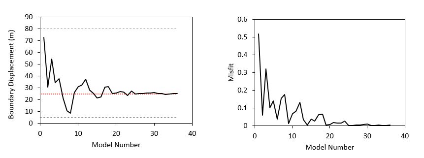
In the present inverse analysis the optimal model corresponds to model number 31 with an optimised boundary displacement of 25.05 m and a misfit value of 0.5732·10-3. Note that in the reference solution the imposed displacement was 25.0 m which means that the present inverse analysis has found an optimal displacement which only has 0.2 % of error relative to the one prescribed in the reference solution. In the following figure it is shown the evolution of the tested boundary displacements and the corresponding misfit values during the inversion analysis.

MEM_003_03

Tested boundary displacements for each model (left) and corresponding misfit value (right). In the figure in the left the value used in the reference solution is shown with the dotted red line whereas the imposed bounds for the inverse analysis are shown in discontinuous grey lines.

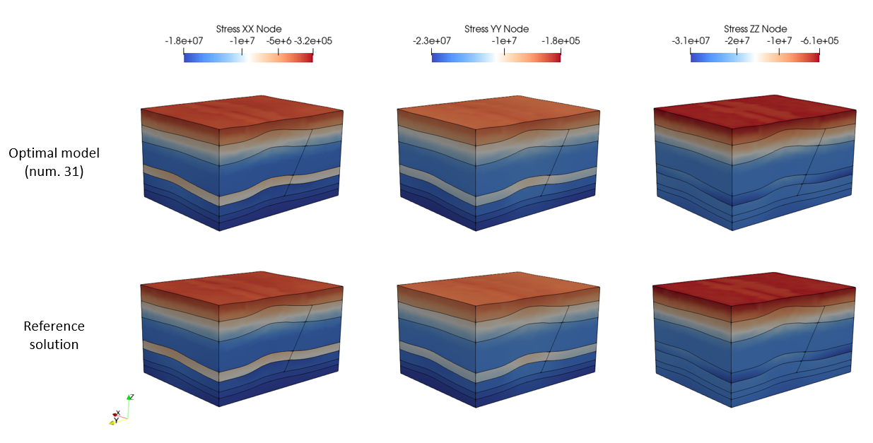
In the folder MEM_003\Case01\Results\Test the data files for all the models run during the inversion analysis are preserved. The optimal model (number 31) has been manually copied and run into the folder MEM_003\Case01\Results\Optimal_Run. The figure below shows the comparison of the optimal model results and the results from the reference solution. As expected the results are almost identical.

MEM_003_02

Stresses plot file comparisons between the optimal model and the reference solution