The initial data file for the project is: geost_002\Data\geost_002_case1.dat. The basic data includes:
1Geometry data (nodes, lines, surfaces and volumes) to define the graben model. The model is 8.5 km long (X direction), 2 km wide (Y direction) and 4 km tall (Z direction). 2Geometry set data (Geometry_set) to group geometry entities into user-named sets and facilitate the assignment of boundary conditions. 3Stratigraphy definition for 4 formations. 4A Stratigraphy_surface_load to define boundary conditions at the top surface. 5Contact data to define contact relationships for surfaces at both sides of faults and detachment (Contact_set, Contact_property and Contact_global). 6Group data for all formations (defined using Group_control_data and Group_data data structures) which are assigned the "Shale_CF75" properties. 7A Material_data structure to read the material properties for the Shale lithology from an external file. 8Data required to define geostatic initialization with a prescribed porosity trend (Geostatic_data, Spatial_variation_definition and Spatial_variation_values ) 9Gravity data (Gravity_data) 10Support data (Support_data) defining fixity in perpendicular directions to each lateral boundary and fixity in vertical direction for the base. 11Mesh control (Mesh_control) and Unstructured mesh generation data (Unstructured_mesh_data) defining a constant mesh size of 300m. 12Damping data (Damping_global_data) to define bulk damping on the effective mean stress (Bulk Viscosity model). 13Time scaling data (Time_scaling_data) with optimal time step 2E-4 Ma. 14History data (History_global) for output of global energy history (results as a function of time). 15Geostatic_control_data to impose elastic constitutive model and elastic contact (no slip) during gravity application. 16Control data (Control_data) defining: a. Incremental solution algorithm (Type 1), b. Duration of t=0.25 Ma, c. Maximum number of time steps 106 (very large to avoid premature termination of the analysis), d. Factor of critical time step = 0.5, e. Plot file output at the end of the stage, f. Screen message output every 500 mechanical steps
Geometry entities may be grouped into geometry sets. This is advantageous when assigning boundary conditions or defining contact relationships for example, where a given condition can be assigned to the whole geometry set (as opposed to the assignment entity by entity). Each defined geometry set may contain any number of lines, surfaces and/or volumes.
Boundary geometry sets
Data File
|
|
* Geometry_set NUM=1
Name "West"
Surfaces IDM=4
8 9 10 11
* Geometry_set NUM=2
Name "East_top"
Surfaces IDM=3
49 50 51
(...)
* Geometry_set NUM=15
Name "Top_surface"
Surfaces IDM=4
7 27 37 52
|
1.Seven geometry sets are defined for boundaries: a. West b.East_top (east boundary above the detachment) c.East_base (east boundary bellow the detachment) d.South e.North f.Base g.Top_surface 2.These geometry sets will facilitate the assignment of boundary conditions (e.g. generally the same boundary condition will be applied to all the surfaces that form part of the North boundary). 3.Surfaces in East_top and East_base could have been included within the same geometry set (the geometry entities of a given geometry set do not need to be contiguous) but have been spited just in case later a prescribed displacement just in the East_top is required (e.g. in order to predict a given lateral stress after initialization without using K0 values).
|
Fault geometry sets
Data File
|
|
* Geometry_set NUM=7
-
Name "fault1_ftw"
Surfaces IDM=3
4 5 6
* Geometry_set NUM=8
Name "fault1_hgw"
Surfaces IDM=3
33 24 23
(...)
* Geometry_set NUM=14
Name "Detachment_hgw"
Surfaces IDM=1
48
|
1Eight geometry sets are defined for faults and detachment (one for the hangingwall and one for the footwall for each fault and detcahment). 2These geometry sets will facilitate the assignment of contact relationships between contact pairs. 3Note that in order to establish contact relationships (e.g. for a fault) the fault must be split in two (hangingwall and footwall parts) otherwise such entity will form part of a continuum.
|
|
The stratigraphy associated with the initial sediment is defined by:
1Defining the existing stratigraphy layer depositional order and the group associated with each layer (via Stratigraphy_definition). 2Defining the topology of the top surface horizon for each stratigraphy layer (via Stratigraphy_horizon). The stratigraphy is defined in a similar way to Mech_002 where a fuller description is provided.
Note that in simulations where geostatic initialization is performed the definition of the stratigraphy is compulsory.
Stratigraphy_definition
Data File
|
|
* Stratigraphy_definition
Unit_Names IDM=4
"formation0"
"formation1"
"formation2"
"formation3"
|
1Four units are present in the initial model. 2Units are specified in depositional order where "formation0" is the oldest unit and "formation3" is the youngest one 3The group names coincide with their respective horizon names and unit names, so only the unit order is required.
|
Stratigraphy_horizon
Data File
|
|
* Stratigraphy_horizon NUM=1
Name "formation0"
Surfaces IDM=2
12 3
* Stratigraphy_horizon NUM=2
Name "formation1"
Surfaces IDM=3
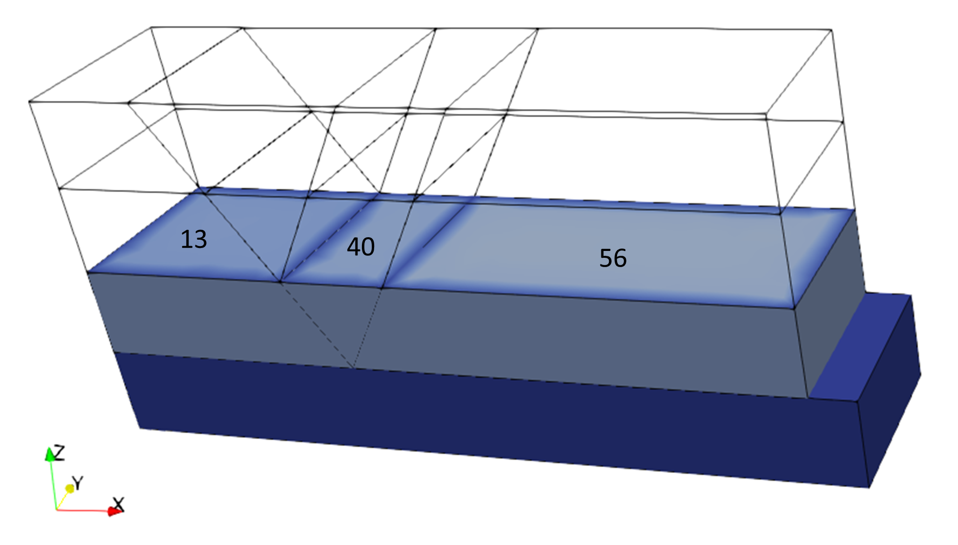
13 40 56
* Stratigraphy_horizon NUM=3
Name "formation2"
Surfaces IDM=4
14 28 41 57
* Stratigraphy_horizon NUM=4
Name "formation3"
Surfaces IDM=4
7 27 37 52
|
1The stratigraphy horizon for each stratigraphy unit must be defined. 2For consistency stratigraphy horizons are named as their respective units (i.e. top surface of formation1 is stratigraphy horizon formation1). 3The top surfaces that define each stratigraphy horizon are specified.

Surface numbers for stratigraphy horizon "formation1"
|
|
A surface load may be defined for the top surface via the Stratigraphy_surface_load data structure. This is usually recommended in coupled problems to prevent the weak sediments near surface to reach positive stresses if pore pressure develops and also in some geomechanical only problems to facilitate stabilization of surface slopes and prevent material flow. In coupled problems boundary conditions for pore pressure and/or temperature may also be specified.
Data File
|
|
* Stratigraphy_surface_load
Applied_stress 0.5
Time_curve_stress "Step_scurve"
|
1A top surface load of 0.5 MPa (effective stress) is applied at top surface. 2The top surface load is ramped up according to an S-curve function during the duration of the present stage (Time_curve_stress set to "Step_scurve")
|
|
The contact data for defining contact relationships for faults and detachment is specified using Contact_set, Contact_property and Contact_global data structures.
Contact_set data structure defines the geometry_sets that can establish contact between each other and will be assigned a given contact property. In addition different options concerning the performance of the contact algorithm are defined.
The Contact_property data structure is used to define the contact models that are used for a given contact set and define the corresponding input properties (e.g. normal penalty stiffnes, tangential penalty stiffnes, coefficient of friction, etc).
The Contact_global data structure is used to define which contact sets are active for the present analysis.
For more information about contact mechanics and contact data definition see Contact Data.
Contact_set
Data File
|
|
* Contact_set NUM=1
Name "All"
Geometry_sets IDM=8
"fault1_ftw"
"fault1_hgw"
"fault2_ftw"
"fault2_hgw"
"fault3_ftw"
"fault3_hgw"
"Detachment_hgw"
"Detachment_ftw"
Algorithm "Penalty"
Property_name "Block_friction"
Global_update_frequency 200
Search_lost_contact 0
Field_factor 0.2
Buffer_factor 0.5
Trigger_search_velocity 10
|
1A single contact set containing all the geometry sets which are expected to establish contact with at least another included geometry set is defined. Any of the included surfaces can establish contact with any of the others unless the permitted surface interaction is defined in Contact_surface data structures. In this example small strain are expected so this is enough (e.g. fault 1 hangingwall is only expected to establish contact with fault 1 footwall). 2The contact algorithm is set to "Penalty" (currently is the only model available). 3The contact set has assigned the contact property named "Block_friction" 4The update frequency for the global contact list (list which stores the facets and nodes which are in contact / will potentially be in contact at a given time of the simulation) is set every 200 mechanical time steps. 5Search lost contact is set to 0 (do not trigger a contact search immediately after contact is lost between two entities). 6The field factor is set to 0.2 (a node and a facet are in contact if the distance between them is 0.2 · lfacet or less, where lfacet is the facet length). 7The buffer factor for defining the buffer box size is set to 0.5 (the candidate target facets that can potentially establish a contact relationship with a given contactor node are those within the buffer box during a global search update). In this case the buffer box for a given node is an sphere centred at the node with radius R=0.5· lfacet where lfacet is the average length of the facets that terminate on the node. 8If a point (node) exceeds the trigger_search_velocity of 10m/Ma (problem units) a global update search will be triggered
|
Contact_property
Data File
|
|
* Contact_property NUM=1
Name "Block_friction"
Compression_model 1
Compression_properties IDM=1
500
Tangential_model 2
Tangential_properties IDM=2
100
0.01
Contact_damping_factor 0.1
|
1A single contact property named "Block_friction" is defined for this example. 2The linear elastic compression model is selected (model 1). 3The normal penalty stiffness is set to 500 MPa. 4The Coulomb friction model is selected for tangential direction (model 2). 5The tangential penalty stiffness is set to 100 MPa and the coefficient of friction is set to 0.01. 6A contact damping factor of 0.1 is set (to facilitate energy dissipation due to contact interaction). |
Contact_global
Data File
|
|
* Contact_global NUM=1
Included_contact_sets IDM=1
"All"
|
A single Contact_global data structure defining the Contact_set named "All" as active is defined.
|
|
The Group_control_data data structure is compulsory and defines:
1The number of geometry groups in the problem, where each geometry group relates to a region with specific properties; e.g. regions with different material assignments, individual stratigraphy layers, etc. 2The group number. 3Whether the group is active or inactive in the fields; i.e. geomechanical, porous flow, thermal, that are being solved.
Data File
|
|
* Group_control_data
Group_numbers IDM=4
1 2 3 4
Active_geomechanical_groups IDM=4
1 1 1 1
|
Four groups are present in the simulation and the geomechanical field is defined as active for such groups.
|
|
The Group_data data structure is compulsory and defines the properties for each geometry group. For this example these comprise:
1The name of the group. 2The element type. 3The material assigned to the group 4The volume that defines the geometry for the group. 5The type of porous flow
Data File
|
|
* Group_data NUM=1
Group_name "formation0"
Element_type TET4V
Material_name "Shale_CF75"
Lumped_storativity_flag 1
Volumes IDM=1
1
Porous_flow_type 5
(...)
* Group_data NUM=4
Group_name "formation3"
Element_type TET4V
Material_name "Shale_CF75"
Lumped_storativity_flag 1
Volumes IDM=4
9 10 11 12
Porous_flow_type 5
|
1Four groups are present in this example and are defined using the TET4V (4 noded tetrahedral elements using the average Volume formulation). 2The material assigned to these element groups is "Shale_CF75". 3The geometry of each group is defined by one or more volumes. 4The simulation will be performed using the porous flow type number 5 (drained simulation with hydrostatic pore pressure in which the effective stress is calculated using the buoyant density). |
|
The material properties for the material "Shale_CF75" are defined in a separate file named Shale.mat. The material_data structure is used to specify the material and material file names.
Data File
|
|
* Material_data NUM=1
Material_name "Shale_CF75"
Material_file "Shale.mat"
|
1A single material is used for the simulation. 2The material is named "Shale_CF75". 3The material properties are defined in Shale.mat file (which should be placed in the same folder as the main model datafile).
|
|
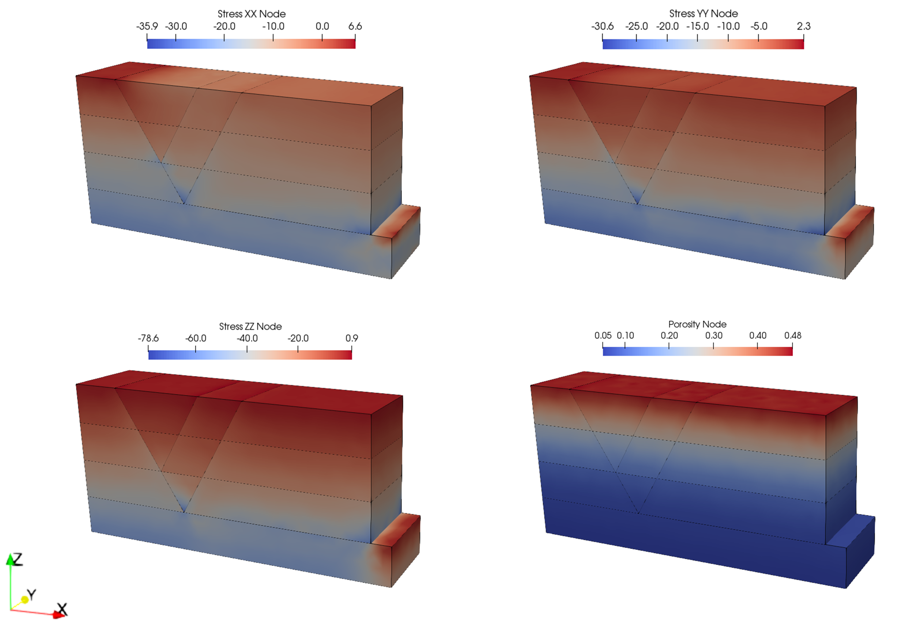
Data for geostatic initialization is defined in the same manner as in the tutorial example geost_001 Initialization of a 3000m 3D column. Full description of the data is provided in Case 1 Base Case description.
Additionally, in this example a Geostatic_control_data data structure enforcing elastic constitutive model and elastic contact (no slip nor separation can occur) during gravity application is included. This data structure is placed before the control stage in the example datafile.
Geostatic_data
Data File
|
|
* Geostatic_data NUM=1
Groups IDM=4
"formation0"
"formation1"
"formation2"
"formation3"
Porosity_spatial 1
Pore_pressure_distribution "Hydrostatic"
Time_curve "Step_scurve"
|
1The geostatic data is applied to the four groups. 2The initial porosity distribution for geostatic initialization will be defined using the Spatial_variation_definition number 1. 3The initial pore pressure distribution will follow an hydrostatic gradient. 4Geostatic initialization will be performed according to a time curve defined by an S-shape function over the duration of the stage (Time_curve set to "Step_scurve")
|
Spatial_variation_definition
Data File
|
|
* Spatial_variation_definition NUM=1
Description "Porosity vs. Depth"
Type "Absolute"
Distribution "Depth_dependent"
Variation_assignment 1
|
1A brief description (164 characters max.) is provided to facilitate identification of the data defined by the spatial variation. 2The type of spatial variation is defined as "Absolute" (i.e. the spatial variation values are absolute values for defining porosity) . 3The distribution is depth dependent (i.e. the spatial variation values will define porosity as a function of depth). 4The Spatial_variation_values data structure number 1 is assigned to define the porosity vs depth trend for initialization. |
Spatial_variation_values
Data File
|
|
* Spatial_variation_values NUM=1
Description "Normal Compaction Trend"
Time 0.0
Values_vs_depth IDM=35 JDM=2
0 179.3 ... 6097.4
0.48834 0.44717 ... 0.039523
|
1A brief description (164 characters max.) is provided to facilitate identification of the data defined by the spatial variation values. 2The time associated for the initialization of the porosity values is set to 0.0 (i.e. from the beginning of the simulation). 3The porosity trend with depth is defined by two rows of 35 depth-ordered values containing: a.Row 1: Depth values b.Row 2: Porosity values |
Gravity_data and associated Time_curve_data
Data File
|
|
* Gravity_data
Gravity_constant 9.810
Time_curve Step_scurve
|
1The gravity constant is defined (9.81 m/s2). 2The Time_curve kwyword is set to Step_scurve so that a smooth s-curve function will be used to apply gravity during the current stage duration. |
Geostatic_control_data
Data File
|
|
* Geostatic_control_data
Stress_constitutive_model "Elastic"
Stress_initialisation_type "Standard"
Contact_constitutive_model "Elastic"
|
1The stress constitutive model is set to elastic (poro-elasticity and/or plasticity for all materials present in the simulation is switched off). 2The stress initialization type is set to "Standard" (stress is initialized according to the data defined in Geostatic_data. This is the default option). 3The contact constitutive model is set to elastic (no slip nor penetration allowed. All other models defined will be switched off).
|
|
The support data is used to define the directions which have the displacement prescribed (in absence of a displacement defined via Global_loads the prescribed displacement is zero, i.e. fixity).
In this example it can be noted the advantage of using geometry sets in order to facilitate the definition of boundary conditions.
Data File
|
|
* Support_data
Displacement_codes IDM=3 JDM=4
1 0 0
0 1 0
0 0 1
1 1 1
Displacement_code_geom_set IDM=6
"West"
"East_top"
"East_base"
"North"
"South"
"Base"
Displacement_code_geom_ass IDM=6
1 1 1 2 2 4
|
1Four sets are defined for definition of combinations of directions for which displacements are constrained/prescribed: (a) Set 1: Displacement prescribed in X direction (b) Set 2: Displacement prescribed in Y direction (c) Set 3: Displacement prescribed in Z direction (d) Set 4: Displacement prescribed in X, Y and Z direction 2The geometry sets which will be assigned one of the displacement code sets defined is listed using Displacement_code_geom_set keyword. 3All geometry sets are prescribed displacement to their respective perpendicular directions (except the base of the model which is fully fixed).
|
|
An "unstructured mesh" with 300m size tetrahedral elements is defined for this example.
Data File
|
|
* Mesh_control_data
Generation_algorithm 2
Mesh_generation_flag 0
* Unstructured_mesh_data
Default_element_size 300
Element_size_bounds IDM=2
300
/ 300
|
1The algorithm used for this simulation is set to 2 (i.e. unstructured mesh). 2The mesh generation flag is set to 0 so analysis will be performed after mesh generation (default). 3The element size is set to 300m.
|
|
Bulk viscosity damping is defined in order to damp the compression part of the dynamics-related oscillations on the effective mean stress.
Data File
|
|
* Damping_global_data
Percentage_damping 0.02000
Bulk_damping_model "BulkViscosity"
Bulk_damping_properties IDM=1
0.5
|
A bulk viscosity model with a bulk viscosity constant of 0.5 is used in this example in order to damp the compressive oscillations due to dynamics in the effective mean stress. This is a generally recommended set up for most of ParaGeo geomechanical analysis. (For more information on the bulk viscosity model see damping_global_data).
Note that despite percentage of damping is defined this will not be active as percentage damping and bulk damping are mutually exclusive and the later has preference.
|
|
The mechanical step size is defined via Time_scaling_factors data structure. The Optimal_time_step keyword has been used. It is the most simple way of defining the mechanical time step size and is generally recommended. Using this method the mass scaling is computed automatically.
Data File
|
|
* Time_scaling_factors
Optimal_time_step 2.0E-04
|
An optimal time step of 2.0·10-4 Ma is defined
|
|
Data File
|
|
* History_global
Output_frequency_time 0.05
Mech_global_energy_data IDM=2
"Kinetic" "Elastic"
|
Output of Kinetic and Elastic energy data is requested every 0.05 Ma
|
|
The current analysis considers a single control stage defined by the Control_data structure in which control data for the geomechanical field is provided. For more information see Solution Control Data.
Data File
|
|
* Control_data
Control_title "Gravity"
Solution_algorithm 1
Maximum_number_time_steps 1000000
Duration 0.25
Factor_critical_time_step 0.5
Output_frequency_plotfile -1
Screen_message_frequency 500
Output_frequency_restart -1
|
1A single control stage of duration 0.25 Ma is defined. 2The solution algorithm is set to number 1, i.e. Transient dynamic algorithm (standard explicit dynamic forward marching algorithm). 3The maximum number of time steps is set to 106. 4The factor critical time step is set to 0.5 so the time step used for the simulation will be 0.5 · 2·10-4. 5Information will be displayed on the screen (command prompt) every 500 mech steps. 6A plot file is requested only at the end of the stage (Output_frequency_plotfile=-1). 7Output of a restart file is requested at the end of the control stage.
|
|
A summary of the data for defining the 3D geometry for this example is presented bellow. These data comprise nodal_data, Geometry_volume, Geometry_surface and Geometry_line data structures.
Nodal_data
Data File
|
|
* nodal_data
node_number IDM=62
1 2 ...
... 62
Coordinates IDM=3 JDM=62
0 0 0
8500 0 0
.
.
.
3600 2000 2000
|
1The 62 nodes that will be used to define geometry lines are defined here. 2The model dimensions are 8500m long x 2000m wide x 4000m tall. 3In 3D problems coordinate Z is for the vertical direction (height/depth).
|
Volumes
Data File
|
|
* geometry_volume NUM=1
Surfaces IDM=7
1 2 3 12 11 15 16
* geometry_volume NUM=2
Surfaces IDM=6
12 4 13 10 17 18
.
.
.
* geometry_volume NUM=12
Surfaces IDM=6
57 51 52 53 62 63
|
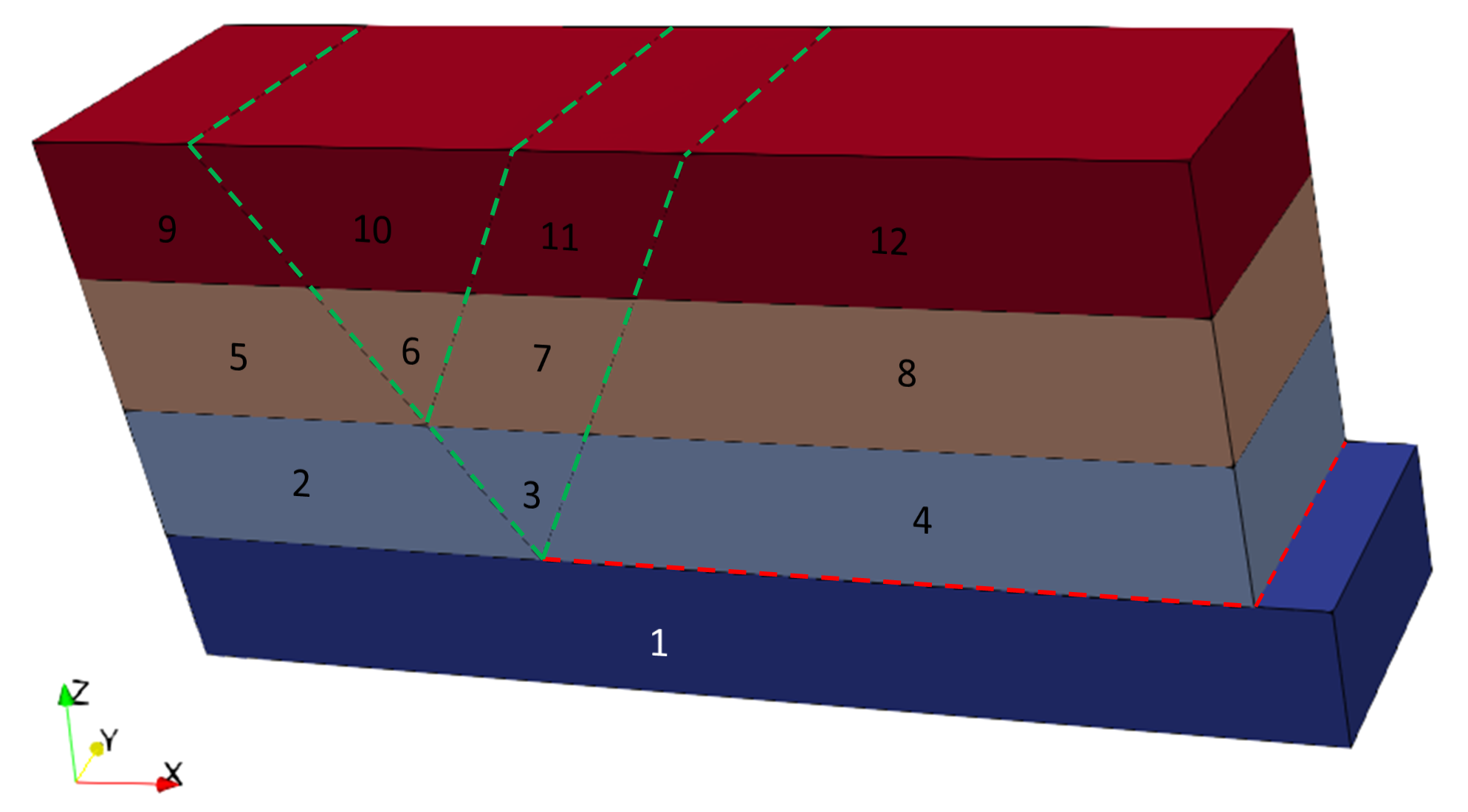
12 volumes define the model geometry.

Volumes that define the graben model geometry
|
Surfaces
Data File
|
|
* geometry_surface NUM= 1
surface_type 5
lines IDM=4
1 80 40 79
* geometry_surface NUM= 2
surface_type 5
lines IDM=4
2 81 41 80
.
.
.
* geometry_surface NUM= 63
surface_type 5
lines IDM=4
78 72 73 74
|
63 surfaces are defined for the current example.
|
Lines
Data File
|
|
* geometry_line NUM=1
points IDM=2
1 2
* geometry_line NUM=2
points IDM=2
2 3
.
.
.
* geometry_line NUM=109
line_type 1
points IDM=2
31 62
|
1109 lines are required to define the current example model's geometry: a.Lines 1 to 39 define the southern boundary of the model (Y=0m) b.Lines 40 to 78 define the northern boundary (Y=2000m) c.Lines 79 to 109 connect each node of the southern boundary with their corresponding northern boundary nodes.
|
|
|

