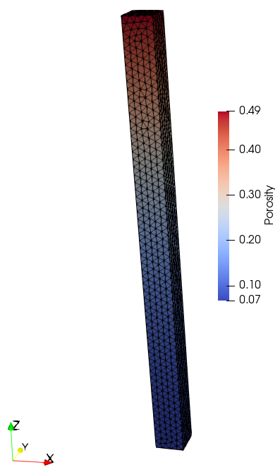
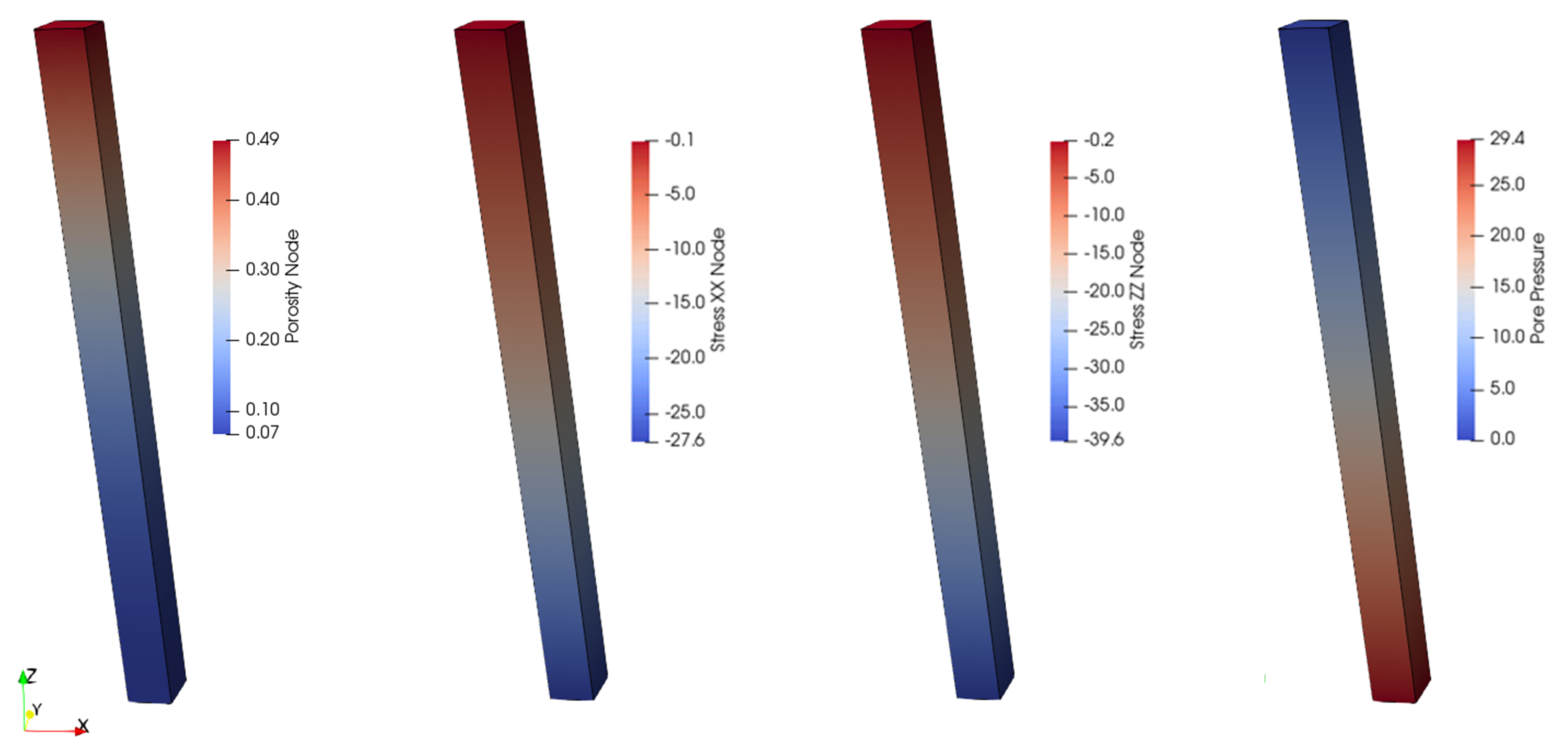
The initial data file for the project is: geost_001\Data\geost_001_case1.dat. The basic data includes:
1Stratigraphy definition for one stratigraphy unit for group "formation0" and the corresponding surface horizon defined by geometry surface 3. 2A Stratigraphy_surface_load to define boundary conditions at the top surface. 3A single group which is assigned the "Shale_CF75" properties defined using Group_control_data and Group_data data structures. 4A Material_data structure to read the material properties for the Shale lithology from an external file. 5Data required to define geostatic initialization with a prescribed porosity trend (Geostatic_data, Spatial_variation_definition and Spatial_variation_values ) 6Gravity data (Gravity_data) 7Support data (Support_data) defining fixity in perpendicular directions to each lateral boundary and fixity in vertical direction for the base. 8Mesh control (Mesh_control) and Unstructured mesh generation data (Unstructured_mesh_data) defining a constant mesh size of 50m. 9Damping data (Damping_global_data) to define bulk damping on the effective mean stress (Bulk Viscosity model) 10Time scaling data (Time_scaling_data) with optimal time step 5E-5 Ma. 11Coupling data (Couple_control_data) to define an incremental coupling between the geomechanical and fluid flow fields using the undrained algorithm. 12History data (History_point and History_global) for output of result history (results as a function of time). 13Control data (Control_data) defining: (a) Incremental Transient solution algorithm (Type 4), (b) Duration of t=1.0 Ma, (c) Factor of critical time step = 0.9, (d) Flow step size of 0.01 Ma (e) Plot file output every 0.2 Ma, (f)Screen message output every 10 flow steps (10 increments) 14Geometry data (nodal_data, Geometry_line, Geometry_surface and Geometry_volume) for definition of the 3D column (200m x 200m x 3000m column).
The stratigraphy associated with the initial sediment is defined by:
1Defining the existing stratigraphy layer depositional order and the group associated with each layer (via Stratigraphy_definition). 2Defining the topology of the top surface horizon for each stratigraphy layer (via Stratigraphy_horizon). The stratigraphy is defined in a similar way to Mech_002 where is a fuller description is provided.
Note that in simulations where geostatic initialization is performed the definition of the stratigraphy is compulsory.
Stratigraphy_definition
Data File
|
|
* Stratigraphy_definition
Unit_Names 1
"formation0"
|
1Only one layer is present in the initial model. 2The group name is "formation0" and the horizon name is "formation0" so only the unit order is required if the unit is also named "formation0".
|
Stratigraphy_horizon
Data File
|
|
* Stratigraphy_horizon NUM=1
Name "formation0"
Lines IDM=1
3
|
1The stratigraphy horizon for unit "formation0" must be defined. 2For consistency it is also named "formation0". 3The top surface of the unit is defined by geometry line 3. |
|
A surface load may be defined for the top surface via the Stratigraphy_surface_load data structure. This is usually recommended in coupled problems to prevent the weak sediments near surface to reach positive stresses if pore pressure develops and in some geomechanical only problems to facilitate stabilization of surface slopes and prevent material flow. In coupled problems boundary conditions for pore pressure and/or temperature may also be specified.
Data File
|
|
* Stratigraphy_surface_load
Applied_stress 0.2
Pore_pressure_flag 1
Time_curve_stress 100
|
1A top surface load of 0.2 MPa (effective stress) is applied to the column. 2Pore pressure is prescribed at top surface by defining Pore_pressure_flag=1 (this is default in coupled problems). 3The top surface load is ramped up according to the rate defined in the load curve number 100 (synchronous to gravity)
|
|
The Group_control_data data structure is compulsory and defines:
1The number of geometry groups in the problem, where each geometry group relates to a region with specific properties; e.g. regions with different material assignments, individual stratigraphy layers, etc. 2The group number. 3Whether the group is active or inactive in the fields; i.e. geomechanical, porous flow, thermal, that are being solved.
Data File
|
|
* Group_control_data
Group_numbers IDM=1
1
Active_geomechanical_groups IDM=1
1
Active_porous_flow_groups IDM=1
1
|
A single group is present in the simulation and the geomechanical and porous flow fields are active for such group
|
|
The Group_data data structure is compulsory and defines the properties for each geometry group. For this example these comprise:
1The name of the group. 2The element type. 3The material assigned to the group 4The volume that defines the geometry for the group. 5The type of porous flow
Data File
|
|
* Group_data NUM=1
Group_name "formation0"
Element_type "TET4V"
Material_name "Shale_CF75"
Volumes IDM=1
1
Porous_flow_type 4
|
1Group 1 is named "formation0" and is defined using the TET4V (4 noded tetrahedral elements using the average Volume formulation). 2The material assigned to this element group is "Shale_CF75". 3The geometry of the group is defined by volume 1. 4The simulation will be performed using the porous flow type number 4 (coupled simulation). |
|
The material properties for the material "Shale_CF75" are defined in a separate file named Shale.mat. The material_data structure is used to specify the material and material file names.
Data File
|
|
* Material_data NUM=1
Material_name "Shale_CF75"
Material_file "Shale.mat"
|
1A single material is used for the simulation. 2The material is named "Shale_CF75". 3The material properties are defined in Shale.mat file (which should be placed in the same folder as the main model datafile).
|
|
The geostatic initialization is performed by:
1Gradual application of gravity to compute the vertical effective stress (Szz'). 2Definition of horizontal effective stress ratios (Sxx'/Szz', Syy'/Szz') for ramping up horizontal effective stresses synchronously to vertical effective stress. 3Assignment of a prescribed initial porosity trend with depth 4Definition of the initial pore pressure distribution with depth

Model initialized with a prescribed porosity vs depth trend
Three data structures are required for the present geostatic initialization: Geostatic_data, Spatial_variation_definition and Spatial_variation_values.
Geostatic_data is the main data structure defining the data for geostatic initialization. In such data structure are defined the list of groups to which the geostatic data is applied, the initial pore pressure distribution, the assignment of a spatial distribution to define the initial porosity vs depth trend, etc. More than one geostatic set may be specified (e.g. to define different geostatic data for different groups present in the simulation).
The porosity vs depth trend is defined using Spatial_variation_definition and Spatial_variation_values data structures. Spatial_variation_definition contains the data to define the type of spatial variation (i.e. absolute, multiplier) and the format input for the values of the spatial variation (i.e. depth dependent, grid). In Spatial_variation_values the values for the spatial variation are defined (e.g. porosity vs depth table).
Geostatic_data
Data File
|
|
* Geostatic_data NUM=1
Groups IDM=1
1
Porosity_spatial 1
Pore_pressure_distribution "Hydrostatic"
k_value_x 0.7
k_value_y 0.7
Time_curve 1
|
1The geostatic data is applied to group 1. 2The initial porosity distribution for geostatic initialization will be defined using the Spatial_variation_definition number 1. 3The initial pore pressure distribution will follow an hydrostatic gradient. 4Horizontal effective stresses in both, X and Y directions will be calculated by multiplying the vertical effective stress by a factor of 0.7. 5Geostatic initialization (pore pressure) will be performed according to the rate described in the time curve number 100 (i.e. synchronous to gravity application. This is generally recommended).
|
Spatial_variation_definition
Data File
|
|
* Spatial_variation_definition NUM=1
Description "Porosity vs. Depth"
Type "Absolute"
Distribution "Depth_dependent"
Variation_assignment 1
|
1A brief description (164 characters max.) is provided to facilitate identification of the data defined by the spatial variation. 2The type of spatial variation is defined as "Absolute" (i.e. the spatial variation values are absolute values for defining porosity) . 3The distribution is depth dependent (i.e. the spatial variation values will define porosity as a function of depth). 4The Spatial_variation_values data structure number 1 is assigned to define the porosity vs depth trend for initialization. |
Spatial_variation_values
Data File
|
|
* Spatial_variation_values NUM=1
Description "Normal Compaction Trend"
Time 0.0
Values_vs_depth IDM=35 JDM=2
0 179.3 ... 6097.4
0.48834 0.44717 ... 0.039523
|
1A brief description (164 characters max.) is provided to facilitate identification of the data defined by the spatial variation values. 2The time associated for the definition of the porosity values is set to 0.0 (i.e. from the beginning of the simulation). 3The porosity trend with depth is defined by two rows of 35 depth-ordered values containing: a.Row 1: Depth values b.Row 2: Porosity values |
Gravity_data and associated Time_curve_data
Data File
|
|
* Gravity_data
Gravity_constant 9.810
Load_curve 100
* Time_curve_data NUM=100
Name "gravity"
Curve_type 2
Time_curve IDM=2
0.0 1.0
Time_factor IDM=2
0.0 1.0
|
1The gravity constant is defined (9.81 m/s2). 2The time curve number 100 is assigned to define the rate for gravity application. 3A name is provided to the time curve to facilitate identification to which load is applied. 4The curve type is set to 2 (i.e. an S-shape curve). 5The time curve is defined in such a way so that from time 0.0 to time 1.0 gravity should be gradually applied following an S-shape function. |
|
The support data is used to define the directions which have a prescribed displacement (in this tutorial example no displacement loads are defined, therefore a direction with a prescribed displacement means that there is fixity in such direction)
Data File
|
|
* Support_data
Displacement_codes IDM=3 JDM=5
1 0 0
0 1 0
0 0 1
1 1 1
0 0 0
Displacement_code_surfaces IDM=6 JDM=2
1 2 3 4 5 6
3 1 5 1 2 2
|
1Five sets are defined for definition of combinations of directions for which displacements are constrained/prescribed: (a) Set 1: Displacement prescribed in X direction (b) Set 2: Displacement prescribed in Y direction (c) Set 3: Displacement prescribed in Z direction (d) Set 4: Displacement prescribed in X, Y and Z direction (e) Set 5: Displacement is free in X, Y and Z directions ( not required as is the default if no displacement code is assigned to a given geometry entity) 2All surfaces are prescribed displacement to their respective perpendicular directions (except top surface which is free to move).
|
|
An "unstructured mesh" with 50m size tetrahedral elements is defined for this example.
Data File
|
|
* Mesh_control_data
Generation_algorithm 2
Mesh_generation_flag 0
* Unstructured_mesh_data
Default_element_size 50
Element_size_bounds IDM=2
50
/ 50
|
1The algorithm used for this simulation is set to 2 (i.e. unstructured mesh). 2The mesh generation flag is set to 0 so analysis will be performed after mesh generation (default). 3The element size is set to 50 m.
|
|
Bulk viscosity damping is defined in order to damp the compression part of the dynamics-related oscillations on the effective mean stress.
Data File
|
|
* Damping_global_data
Percentage_damping 0.02000
Bulk_damping_model "BulkViscosity"
Bulk_damping_properties IDM=1
0.50000
|
A bulk viscosity model with a bulk viscosity constant of 0.5 is used in this example in order to damp the compressive oscillations due to dynamics in the effective mean stress. This is a generally recommended set up for most of ParaGeo geomechanical analysis. (For more information on the bulk viscosity model see damping_global_data).
Note that despite percentage of damping is defined this will not be active as percentage damping and bulk damping are mutually exclusive and the later has preference.
|
|
The mechanical step size is defined via Time_scaling_factors data structure. The Optimal_time_step keyword has been used. It is the most simple way of defining the mechanical time step size and is generally recommended. Using this method the mass scaling is computed automatically.
Data File
|
|
* Time_scaling_factors
Optimal_time_step 5.0E-05
|
An optimal time step of 5.0·10-5 Ma is defined
|
|
Couple_control_data is a compulsory data structure for coupled simulations. The minimum data required is the specification of the fields active in the coupling. In this example data for specification of the solution algorithm, the volume strain coupling model and the volume update model is also defined.
Data File
|
|
* Couple_control_data
Solution_algorithm "Incremental"
Volume_strain_coupling "Undrained"
Volume_update_model "VariableGroup"
Field_names IDM=2
"Geomechanical"
"Porous_flow"
|
1The solution algorithm to be used for the coupling is incremental (one iteration). 2The "Undrained" model is used for coupling of the volumetric strain. This is recommended for the analysis of low permeability formations (e.g. clays, shales). 3The "VariableGroup" model for computation of the bulk stiffness for the mechanical field is selected (for more information see Couple_control_data). 4The fields that will be coupled are Geomechanical and Fluid Flow. |
|
Two types of history output data structures are used in this example. The History_point data structure is used to output data for selected variables for a specified location within the problem domain. The History_global data structure is used to output global energy data.
History_point
Data File
|
|
* History_point NUM=1
Name "Set1"
Group 1
Output_frequency_time 0.05
Point_coordinates IDM=3 JDM=1
100 100 100
Displacements IDM=2
"DISP_X" "DISP_Y"
Stresses IDM=3
"STRS_XX" "STRS_YY" "STRS_ZZ"
Stress_invariants IDM=2
"PRESS" "EFSTRS"
Element_data IDM=2
"POROSITY" "ELT_PORE"
Elastic_state_variables IDM=1
"YOUNG"
Plastic_state_variables IDM=7
"P_STRN" "P_STRNV" "P_STRNXX" "P_STRNYY"
"P_STRNZZ" "P_COMC" "P_TENC"
Strain_invariants IDM=2
"Vol_stn" "Efstrn"
|
1A history point named "Set 1" is defined at X=100m, Y=100m, Z=100m location to output data every 0.05 Ma for the selected variables 2A list of selected variables for output data is provided. For more information about the syntax for the output variables see History_point.
|
History_global
Data File
|
|
* History_global
Output_frequency_time 0.01
Mech_global_energy_data IDM=2
"Kinetic" "Elastic"
|
Output of Kinetic and Elastic energy data is requested every 0.01 Ma
|
|
The current analysis considers a single control stage defined by the Control_data structure in which control data for both the geomechanical and fluid flow fields is provided. For more information see Solution Control Data.
Data File
|
|
* Control_data
Control_title "init_0"
Duration 1.0
Solution_algorithm 4
Maximum_number_time_steps 100000
Initial_time_increment 0.005
Maximum_number_iterations 5000
Factor_critical_time_step 0.6
Screen_message_frequency 10
Output_frequency_plotfile -1
Output_time_plotfile 0.2
Output_frequency_restart -1
Output_time_restart 0.0
|
1A single control stage of duration 1 Ma is defined. 2The solution algorithm is set to number 4, i.e. Incremental Transient (compulsory for coupled simulations). 3The maximum number of time steps is set to 105. 4The flow step size (coupling step) is set to 0.005 Ma. 5The maximum number of iterations is set to 5000 (very high). 6The factor critical time step is set to 0.6 so the time step used for the simulation will be 0.6 · 5·10-5. 7Information will be displayed on the screen (command prompt) every 10 flow steps. 8A plot file is requested every 0.2 Ma (Output_time_plotfile=0.2) and at the end of the stage (Output_frequency_plotfile=-1). 9Output of a restart file is requested at the end of the control stage. |
|
A summary of the data for defining the 3D geometry for this example is presented bellow. These data comprise nodal_data, Geometry_volume, Geometry_surface and Geometry_line data structures.
Nodal_data
Data File
|
|
* nodal_data
node_number IDM=8
1 2 3 4 5 6 7 8
coordinates IDM=3 JDM=8
0.0 0.0 0.0
200 0.0 0.0
200 0.0 3000
0.0 0.0 3000
0.0 200 0.0
200 200 0.0
200 200 3000
0.0 200 3000
|
1All the nodes that will be used to define geometry lines are defined here. 2The geometry is a rectangular prism (3D column) so 8 nodes are required. 3In 3D problems coordinate Z is for the vertical direction (height/depth). 4The nodes for a 200m x 200m x 3000m column are defined.
|
Volumes
Data File
|
|
* geometry_volume NUM=1
Surfaces IDM=6
1 2 3 4 5 6
|
A single volume formed by 6 surfaces defines the geometry of the problem.
|
Surfaces
Data File
|
|
* geometry_surface NUM=1
surface_type 5
lines IDM=4
1 10 5 9
* geometry_surface NUM=2
surface_type 5
lines IDM=4
2 11 6 10
.
.
.
* geometry_surface NUM=6
surface_type 5
lines IDM=4
5 6 7 8
|
1Six surfaces are defined (Base, top surface and 4 lateral surfaces). 2Each surface is defined by four lines.
|
Lines
Data File
|
|
* geometry_line NUM=1
line_type 1
points IDM=2
1 2
* geometry_line NUM=2
line_type 1
points IDM=2
2 3
.
.
.
* geometry_line NUM=12
line_type 1
points IDM=2
4 8
|
1Twelve lines are defined (4 for the base, 4 for the top surface and 4 that connect each corner of the base with the respective corner of the top surface). 2Each line connect two nodes.
|
|
|


