The present example demonstrates the set up of a Material Earth Model (MEM) simulation encompassing the initialization which is performed in several stages followed by two production stages. Initial values for porosity and pore pressure are defined at element basis via Spatial_grid data structures. The simulation is geomechanical only with all changes in pore pressure being prescribed.
The data files for the project are in: MEM_002\Case01\Data. The data comprises:
1.MEM_002_Case01.dat: Main problem data file.
2.MEM_002_Case01.geo: Geometry and mesh for the problem.
3.MEM_002_Case01.geometry: Data file with definition of geometry sets and groups for the problem
4.MEM_002.mat: Material file including Material_data for all lithologies
5.MEM_002_Case01_Porosity.spat: File containing a Spatial_grid with the initial element porosity values for all formations.
6.MEM_002_Case01_PP_Initial.spat: File containing a Spatial_grid with the initial element pore pressure values for all formations.
7.MEM_002_Case01_PP_2021.spat: File containing a Spatial_grid with the element pore pressure values at the end of year 2021 for the reservoir formation.
8.MEM_002_Case01_PP_2022.spat: File containing a Spatial_grid with the element pore pressure values at the end of year 2022 for the reservoir formation.
The different simulation stages and the operations performed are described below.
Stage 1: Elastic Gravity Initialization
•Gravity is ramped up during the duration of the stage.
•Initial porosities for the formations is defined via a spatial grid with element values.
•Materials are kept elastic.
•Young modulus for the "Reservoir" formation is defined as a function of porosity using a Spatial_table.
•Horizontal stress increases as a function of vertical stress and Poisson's ratio.
•Initial pore pressure distribution is defined via a spatial grid with element values.
•Initial temperature distribution is defined according to a surface temperature and a temperature gradient.
•The initial units for salt viscosity are 10000 s of years (dka)
Stage 2: Tectonic Displacement
•A tectonic displacement load is applied in order to obtain the in-situ horizontal stress.
•Materials are kept elastic.
Stage 3: Constitutive Release
•Constitutive models are switched from "Elastic" to "Standard".
•Final stresses at the end of the previous stage are saved and ramped up from zero during the present stage.
•Pore pressure is ramped up from zero.
•Displacement is reinitialized.
Stage 4: Time Units Update (10K years to 100 years)
•Time units for the salt viscosity are updated from 10000 s of years (dka) to 100 s of years (cyears).
•Final stresses at the end of the previous stage are saved and ramped up from zero during the present stage.
•Pore pressure is ramped up from zero.
•Displacement is reinitialized.
Stage 5: Time Units Update (100 s years to years)
•Time units for the salt viscosity are updated from 100 s of years (cyears) to years.
•Final stresses at the end of the previous stage are saved and ramped up from zero during the present stage.
•Pore pressure is ramped up from zero.
•Displacement is reinitialized.
Stage 6: Time Units Update (years to days)
•Time units for the salt viscosity are updated from years to days.
•Final stresses at the end of the previous stage are saved and ramped up from zero during the present stage.
•Pore pressure is ramped up from zero.
•Displacement is reinitialized.
Stage 7: 1st Year of Production
•A pore pressure decrease of 12·106 Pa in the reservoir is imposed via a spatial grid with element values and usage of a Spatial_boundary.
Stage 8: 2nd Year of Production
•A pore pressure decrease of 8·106 Pa in the reservoir is imposed via a spatial grid with element values and usage of a Spatial_boundary.
Following there is the description of the data file. The first section named "Model Definition Data" describes the data defining the model which is not related to initialisation or production (e.g. geometry, mesh, groups, etc). Subsequently the data relative to each of the stages is described.
Model Definition Data
Here the data defining the model which is not related to initialisation or production is described. Note that the data may not be described in the same order as it appears in the data file.
Geometry and Mesh
The mesh for the model was generated using Gmsh and exported to Abaqus format. Then the Abaqus --> ParaGeo conversion was used to generate the geometry stored in the MEM_001_Case01.geo file.
Data File
|
|
* Geometry_data
File_name MEM_001_Case01.geo
File_format hdf
* Include
Filename MEM_001_Case01.geometry
|
1.The geometry and mesh for the model is read from the .geo file using the Geometry_data structure.
2.An Include data structure is used to incorporate to the main problem data file the data defined in the .geometry file which contains data for the groups and geometry sets. |
Data File
|
|
* Geometry_set NUM=1
Name "Base"
Set_type "Abaqus NSET"
Surfaces IDM=1
7
* Geometry_set NUM=2
Name "South"
Set_type "Abaqus NSET"
Surfaces IDM=7
8 9 10 11 12 13 14
(...)
* Geometry_set NUM=19
Name "Shale04"
Set_type "Group"
Volumes IDM=1
7
|
1.The .geometry file contains 19 Geometry_set data structures defining model boundaries, stratigraphy horizons and groups. |
Group data
Data File
|
|
* Group_control_data
Group_numbers IDM=7
1 2 3 4 5 6 7
Active_geomechanical_groups IDM=7
1 1 1 1 1 1 1
* Group_data NUM=1
Group_name "Shale01"
Element_type "Tet4v"
Material_name "Shale"
Porous_flow_type 2
Volumes IDM=1
1
Geometry_set "Shale01"
Average_pressure_flag 0
* Group_data NUM=2
Group_name "Salt01"
Element_type "Tet4v"
Material_name "Salt_Pa_dKa"
Porous_flow_type 2
Volumes IDM=1
2
Geometry_set "Salt01"
Average_pressure_flag 1
(...)
|
1.A Group_data data structures is defined for each of the seven formations.
2.Group_control_data is used to define geomechanical field active for the seven formations.
3.Element_type is set to TET4V (4 node 3D tetrahedral elements with average volume formulation) and each formation is assigned the appropriate material data (which is defined in the included .mat file).
4.Porous_flow_type is set to 2 (mechanical analysis with prescribed pore pressure).
5.The volume and Geometry_set defining the group are specified. Note that both are equivalent and only one of those is required. However both are included here as is how the data was obtained after mesh conversion from Gmsh (using the Abaqus --> ParaGeo conversion).
6.The two salt formations have the Average_pressure_flag set to 1 in order to obtain a smooth stress field. |
Materials
The materials are defined in a separate file named MEM_001_Case01.mat which is included in the main datafile using the command Include. The properties for the different lithologies are defined so that:
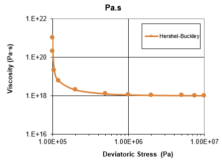
•Salt is modelled with Herschel-Bulkley viscoplastic properties with parameters targeting a viscosity of the order of 1·1018 Pa·s for relatively high stresses (106 Pa = 1 MPa). •Shale formations are elastic. Deeper shale formations have higher Young modulus values than shallower shale formations. •Reservoir formation is poro-elastic.
Data File
|
|
* Material_data
Material_name "Salt_Pa_dKa"
Units IDM=4
"Pa"
"m"
"dka"
"Celcius"
Grain_stiffness 70000E6
Grain_density 2200.00
Porosity_model_type 1
Porosity 0.02
Elastic_model_type 1
Elastic_properties IDM=2
18.1E+9
0.265
Viscoplastic_material_type 1
Viscoplastic_properties IDM=3
100000
3.2E+6
1.0
Singlephase_fluid_name "Water"
* Material_data
Material_name "Shale01"
Grain_stiffness 20000E6
Grain_density 2650.00
Porosity_model_type 1
Porosity 0.30
Elastic_model_type 1
Elastic_properties IDM=2
2500.0E6
0.35
Singlephase_fluid_name "Water"
* Material_data
Material_name "Reservoir"
Grain_stiffness 20000E6
Grain_density 2450.00
Porosity_model_type 1
Porosity 0.35
Elastic_model_type 1
Elastic_properties IDM=2
2000.0E6
0.20
Porous_elasticity_type 1
Porous_elastic_properties IDM=2
10.0E+6
0.02
Singlephase_fluid_name "Water"
|
1.Material units are specified for all lithologies (not shown).
2.Salt initial porosity is defined very low and consequently salt Young's modulus is defined close to the grain stiffness value.
3.Viscoplastic_material_type is set to 1 (Herschel-Bulkley).
4.Viscoplastic properties are defined so that the yield stress is set to 105 Pa (0.1 MPa) and the viscosity at large stresses is approximately asymptotic to 1·1018 Pa·s as shown below:

Salt viscosity in Pa·s as a function of deviatoric stress.
5.It should be noted that initially the salt viscosity is defined in 10000 s of years units (dka) as stated in the initial problem units. Note however that the value will be scaled as we gradually update the problem time units to production time frames (days) during initialization. This is done because during initialization we want to achieve a stress state close to an isotropic state within the salt. Thus the larger mobility of salt over dka time frames facilitates that whereas during production we are interested to represent salt mobility over a time frame of days (actual observed response upon production).
6.Only one shale lithology Material_data is shown here as the different shales only differ on the Young's modulus value which is: ▪Shale01: 2500·106 Pa ▪Shale02: 2000·106 Pa ▪Shale03: 1500·106 Pa ▪Shale04: 1000·106 Pa
7.The Porosity value (reference porosity) will be overwritten by values prescribed using the Spatial_grid.
8.Reservoir formation is defined poroelasticity data. |
Stratigraphy data
For MEM applications definition of the complete stratigraphy is not required but only definition of the top surface. This enables to perform geostatic initialization and any depth-based calculation (e.g. output of element depth variable to plot file, definition of initial temperature as a function of depth).
Data File
|
|
* Stratigraphy_definition
Top_surface_horizon "Top"
* Stratigraphy_horizon NUM=1
Name "Top"
Geometry_set "Shale04_top"
* Stratigraphy_surface_load
Applied_stress 100000.0
Time_curve_stress "Step_scurve"
* Stratigraphy_smoothing
Active_flag -1
|
1.Stratigraphy_definition and Stratigraphy_horizon are used to identify the top surface (defined by the geometry set "Shale04_top").
2.A stress load of 1·105 Pa is applied to the top surface. The load is ramped up synchronous to the gravity following an s-curve function over the duration of the stage.
3.Stratigraphy smoothing is off during the simulation (Active_flag set to -1). |
Support data
Data File
|
|
* Support_data
Displacement_codes IDM=3 JDM=3
1 0 0
0 1 0
0 0 1
Displacement_code_geom_set IDM=5
"East"
"West"
"North"
"South"
"Base"
Displacement_code_geom_ass IDM=5
1 1 2 2 3
|
1.Displacements are constrained in the normal direction for the Base and side boundaries. |
|
Additional Data Output
Here the data used to request additional output to the plot file output defined within Control_data is described. The additional data output includes:
1.One history point set with one point at each formation for monitoring initialization 2.Two history points sets for monitoring changes during production 3.Two history line output (History_section_line) to output displacement profile at the top surface. 4.A reference set to request output of change in selected variables during production
Initialization Stages
Data File
|
|
* History_point NUM=1
Name "Initialization"
Output_frequency_time 0.01
Point_labels IDM=7
"Shale01"
"Salt01"
(...)
"Shale04"
Point_coordinates IDM=3 JDM=7
5600 7900 1300
5600 7900 1750
(...)
5600 7900 5600
Displacements IDM=3
"Disp_x" "Disp_y" "Disp_z"
Velocities IDM=3
"Veloc_x" "Veloc_y" "Veloc_z"
(...)
Viscoplastic_state_variables IDM=5
"V_strn" "V_strn_r" "V_strnv" "V_strs" "V_viscos"
|
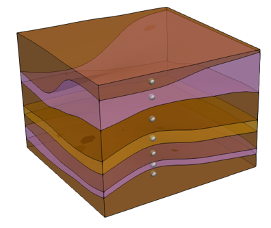
1.A History_point data structure is used to monitor the evolution of the specified variables during initialization.
2.There is one point defined for each of the formations next to the North boundary as shown in the image below. 
Location of history points for monitoring initialization stages
|
Production Stages
Data File
|
|
* Reference_set_data NUM=1
Name "Production"
Output_change 1
Groups IDM=7
"Shale01"
"Salt01"
"Shale02"
"Reservoir"
"Shale03"
"Salt02"
"Shale04"
Nodal_variables IDM=1
"Disp"
Element_variables IDM=6
"Porosity" "Effmean" "Vonmises"
"Strs_xx" "Strs_yy" "Strs_zz"
* History_point NUM=1
Active_flag -1
* History_point NUM=2
Name "Reservoir"
Group_name "Reservoir"
Output_frequency_time 1.0
(...)
* History_point NUM=3
Name "Seal"
Group_name "Shale03"
Output_frequency_time 1.0
(...)
* History_section_line NUM=1
Name "SubsidenceY"
Output_frequency_increment -1
Point_distribution_type 0
Point_distance 100
Path_coordinates IDM=3 JDM=2
5600 8000 5940
5600 0 5940
Displacements IDM=1
"Disp_z"
* History_section_line NUM=2
Name "SubsidenceX"
Output_frequency_increment -1
Point_distribution_type 0
Point_distance 100
Path_coordinates IDM=3 JDM=2
0 7900 5940
8000 7900 5940
Displacements IDM=1
"Disp_z"
|
1.A Reference_set_data is defined at the first production stage so that the change in the specified variables is output to the plot file. Because the data is named "Production" the output variables will be named according to the following format: "Production Delta Porosity".
2.The history output for the history point set number 1 (defined to monitor initialization) is requested to stop via Active_flag set to -1. This is done to avoid too many outputs resulting from the different duration for production stages (note that Output_frequency_time for history point set was set to 0.01 time units and the production stages have a duration of 365 days each).
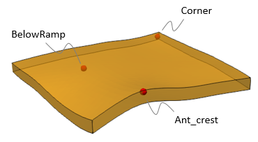
3.Two History_point set data structures are defined to monitor evolution of selected variables during production. The objective ob each History_point set is to monitor evolution of specified properties at: a.Three different reservoir locations (see image below) b.Seal above the reservoir anticline crest (just above the Ant_crest point in the image below)

Reservoir history points locations to monitor production stages. Point labels are indicated.
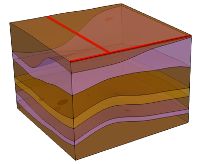
4.Two History_section_line data structures are defined to output top surface vertical displacement (subsidence) along X and Y axis both crossing point (x, y) = (5600, 7900) located above the anticline crest where a producer well will be placed in next examples (see image below). Note that: a.The data is defined at the last stage of initialization so that the initial displacement before production may be subtracted to calculate the increments. b.Output is performed at the end of each stage (Output_frequency_increment set to -1). c.Output is performed every 100 m (Point_distance set to 100).

Location of the history section lines.
|
|
Stage 1: Elastic Gravity Initialization Data
Definition of initial Units
In the present case definition of Units is relevant for two reasons:
1.It allows to define gravity as 9.81 m/s2 and the code will perform the corresponding scaling according to the units chosen.
2.To set the initial time units for the defined salt viscosity in the Material_data. This allows to later update the time units and the code will automatically scale viscosity accordingly. Note that we are interested to initialise salt with properties at geological time scale so that at initial isotropic stress state within the salt is achieved. Otherwise the viscosity may be to high and large deviatoric stresses may be retained within the salt. Later we are going to gradually change time units so that during production stages we have properties that are appropriate for the time scale.
Data File
|
|
* Units
Length "m"
Stress "Pa"
Time "dka"
Temperature "Celsius"
Permeability "m^2"
Conductivity "W"
|
1.The Units for the problem are defined. In the present case definition of units is relevant for two reasons: a.Gravity will be specified as 9.81 m/s2 and the code will perform the corresponding scaling according to the units chosen. b.To set the initial time units for the defined salt viscosity. This allows to later update the time units and the code will automatically scale viscosity accordingly. Note that
|
Gravity data
Data File
|
|
* Gravity_data
Gravity_constant 9.81
Time_curve "Step_scurve"
|
1.Gravity_data is defined with an assigned internally generated s-curve time curve. |
Geostatic data and definition of initial porosity
The initial porosity distribution for shale and reservoir formations is defined at an element basis via a Spatial_grid and prescribed using Geostatic_data. Geostatic_control_data is used to define the initialization options for the current stage.
Data File
|
|
* Geostatic_control_data
Description "Gravity_Load"
Stress_constitutive_model "Elastic"
Stress_initialisation_type "Standard"
Viscoplastic_model "Elastic"
Displacement_reinit_flag 0
State_reinit_flag 0
Time_curve "Step_scurve"
* Geostatic_data NUM=1
Name "Initialisation"
Groups IDM=5
"Shale01"
"Shale02"
"Shale03"
"Shale04"
"Reservoir"
Porosity_spatial_grid "Porosity"
* Include
Filename MEM_001_Case01_Porosity.spat
* Spatial_grid NUM=4
Name "Porosity"
Type "Element"
Element_variables IDM=1
"Porosity"
Element_numbers IDM=66090
1 2 ...
... 66089 66090
Element_values IDM=1 JDM=66090
0.14353
0.14959
(...)
0.54510
|
1.In Geostatic_control_data the options for the current initialization stage are defined: a.The materials will be kept elastic (Stress_constitutive_model set to Elastic) b.The stresses are initialized with gravity (Stress_initialization_type set to standard) c.No displacement re-initialization nor state variable re-initialization is performed (respective flags set to 0)
1.The Spatial_grid defining element porosity values is defined in a separate file named MEM_001_Case01_Porosity.spat which is included by using the data structure Include.
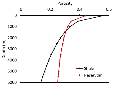
2.The Spatial_grid contains values for the element variable "Porosity" for the 66090 elements of the domain. The element numbers and their corresponding porosity values are specified. The porosity curves used to define the grid are shown in the image below.
3.Geostatic_data is defined in order to use the values defined in the spatial grid named "Porosity" to prescribe the initial porosity values. Note that the two salt formations are not defined an initial porosity via the Spatial_grid and Geostatic_data as they are using the reference porosity defined in the corresponding Material_data.
4.It should be noted that initial porosity values could also be prescribed using a Spatial_state_set and assigning the porosity grid instead of using Geostatic_data. Nonetheless usage of Geostatic_data is generally preferred because in cases involving plastic materials with hardening, the initial plastic volumetric strain should be evaluated from the initial porosity value and the reference porosity in order to obtain an appropriate initial value for pre-consolidation pressure (this procedure is only invoked when using Geostatic_data).

Compaction curves used to define the porosity grid
|
Definition of initial Pore Pressure
The initial pore pressure distribution for the whole domain is defined via a Spatial_grid and prescribed using the Spatial_boundary.
Data File
|
|
* Include
Filename MEM_001_Case01_PP_Initial.spat
* Spatial_grid NUM=4
Name "Pore_Pressure_Init"
Type "Element"
Element_variables IDM=1
"Elt_pore"
Element_numbers IDM=66090
1 2 ...
... 66089 66090
Element_values IDM=1 JDM=66090
0.10161E+09
0.96442E+08
(...)
0.23901E+07
* Spatial_boundary NUM=1
Name "Pore Pressure"
Boundary_type "Spatial_grid"
Value_type "Absolute"
Mapping_entity_flag 0
Spatial_grids IDM=1
"Pore_Pressure_Init"
Prescribed_components IDM=1 JDM=1
6
Time_curve "Step_scurve"
|
1.The Spatial_grid defining element pore pressure values is defined in a separate file named MEM_001_Case01_PP_Initial.spat which is included by using the data structure Include.
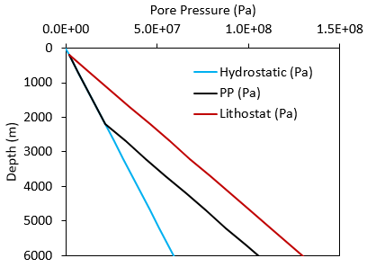
2.The Spatial_grid "Pore_pressure_Init" contains values for the element variable "Elt_pore" for the 66090 elements of the domain. The element numbers and their corresponding pore pressure values are specified. The pore pressure profile used to define the grid is shown in the figure below.
3.The Spatial_boundary data structure is defined in order to use the values defined within the "Pore_Pressure_Init" spatial grid to prescribe the initial pore pressure at element basis (Prescribed_components set to 6). Note that the initial pore pressure will be gradually ramped up from zero synchronous to gravity following an s-curve over the duration of the stage.

Pore pressure distribution with depth defined via the spatial grid
|
Temperature Distribution
The initial temperature distribution is defined via a Global_loads and a Spatial_variation_definition
Data File
|
|
* Global_loads NUM=1
Name "Temperature vs. Depth"
Prescribed_temperature IDM=1 JDM=1
1.0
Prescribed_temperature_spatial 1
Pres_temperature_geom_set IDM=1
"All_volumes"
Pres_temperature_geom_ass IDM=1
1
* Spatial_variation_definition NUM=1
Description "Temperature vs. Depth"
Type "Absolute"
Distribution "Depth_dependent"
Variation_assignment 1
* Spatial_variation_values NUM=1
Description "Temp. vs. Depth"
Time 0.0
Values_vs_depth IDM=2 JDM=2
0.0 20960.5
10.0 534.013
* Time_curve_data NUM=1
Name "Temperature"
Time_curve IDM=2
0.0 1.0
Time_factor IDM=2
1.0 1.0
Curve_type 1
* Load_case_control_data
Loadcases IDM=1
1
Active_load_flags IDM=1
2
|
1.A Global_loads data structure is defined to prescribe a spatial distribution of temperature.
2.A single Prescribed_temperature set is defined with its value being set to 1.0. Note that this will not be used as the spatial distribution will be used instead.
3.Prescribed_temperature_spatial is assigned Spatial_variation_definition number 1.
4.The prescribed temperature set is assigned to "All_volumes" geometry set (a reserved geometry set generated by the code that encompasses all the volumes in the domain).
5.The Spatial_variation_definition and Spatial_variation_values defining the temperature distribution with depth.
6.The temperature is prescribed as an instantaneous load. The values are defined according to a surface temperature of 10 ºC and a temperature gradient of 0.025 ºC/m. |
Control data
Data File
|
|
* Control_data
Control_title "init"
Solution_algorithm 1
Initial_time_increment 1.0
Displacement_norm_tolerance 0.01
Residual_norm_tolerance 0.01
Duration 1.0
Target_number_time_steps 10000
Output_frequency_plotfile -1
Output_time_plotfile 0.2
Output_frequency_restart -1
Screen_message_frequency 1000
|
1.Control_data data structure defines solution data for the stage.
2.All stages have identical control data so that only the present stage will be described. The key data comprises: a.Solution_algorithm set to 1 (transient dynamic algorithm) which is compulsory for geomechanical only simulations. b.Duration is set to 1.0 time units c.The Target_number_time_steps is set to 10000 (which defines the target number of mechanical steps to solve the stage). d.Simulation information will be printed to the command prompt every 1000 mech steps (Screen_message_frequency set to 1000). e.A plot file will be output every 0.2 time units (Output_time_plotfile set to 0.2) and at the end of the stage (Output_frequency_plotfile set to -1) f.A restart file will be output at the end of the stage (Output_frequency_restart set to -1) |
|
Stage 2: Tectonic Displacement
Geostatic Options
Data File
|
|
* Geostatic_control_data
Description "Tectonic"
Stress_constitutive_model "Elastic"
Stress_initialisation_type "None"
Viscoplastic_model "Elastic"
Displacement_reinit_flag 0
State_reinit_flag 0
Time_curve "Step_constant"
* Spatial_boundary NUM=1
Name "Pore Pressure"
Boundary_type "Spatial_grid"
Value_type "Absolute"
Mapping_entity_flag 0
Spatial_grids IDM=1
"Pore_Pressure_Init"
Prescribed_components IDM=1 JDM=1
6
Time_curve "Step_constant"
|
1.In Geostatic_control_data the options for the current stage are defined: a.Materials are kept elastic b.Stresses are not initialised (values calculated from the previous stage are kept as the initial values) c.No displacement re-initialization nor state variable re-initialization is performed (flags set to 0)
2.Spatial_boundary needs to be re-specified in order to consider the initial pore pressure values defined by the spatial grid. Because we are not interested in re-initializing the values during this stage (as we do not re-initialize stresses) a "Step_constant" curve is assigned (constant factor of 1.0 over the duration of the stage). |
Tectonic Load
Data File
|
|
* Global_loads NUM=2
Name "Tectonic_disp"
Prescribed_displacement IDM=3 JDM=1
1.0 0.0 0.0
Pres_displacement_geom_set IDM=1
"West"
Pres_displacement_geom_ass IDM=1
1
* Time_curve_data NUM=2
Name "Tectonic_disp"
Time_curve IDM=2
1.0 2.0
Time_factor IDM=2
0.0 20.0
Curve_type 2
* Load_case_control_data
Loadcases IDM=2
1 2
Active_load_flags IDM=2
2 2
|
1.A prescribed displacement of 20 m is applied to the "West" boundary. This is achieved by: a.Defining a Global_loads data structure with a prescribed displacement set with a displacement of 1.0 m in the X direction. b.Assigning the displacement set to "West" boundary. c.Defining a multiplication factor of 20.0 in the corresponding time curve.
2.The Global_loads number 2 defining the tectonic displacement is defined as active (flag = 2) as well as Global_loads number 1 corresponding to the temperature load.
|
|
Stage 3: Constitutive Release and Time Units Update
Geostatic Options
Data File
|
|
* Geostatic_control_data
Description "Release"
Stress_constitutive_model "Standard"
Stress_initialisation_type "Standard"
VIscoplastic_model "Standard"
Displacement_reinit_flag 1
Poroelastic_init_flag 1
State_reinit_flag 0
Time_curve "Step_scurve"
|
1.In Geostatic_control_data the options for the current stage are defined: a.Materials are using the constitutive properties as defined in Material_data (Stress_constitutive_model set to "Standard"). b.Stresses are re-initialised (Stress_initialisation_type set to "Standard") c.Displacement is re-initialized so that the geometry will go back to the state prior to any compaction. d.Porelastic_reinit_flag set to 1 indicates that the stresses at the end of the previous stage are used to evaluate poroelastic constants (i.e. Bulk modulus) otherwise because we are re-initializing stresses the initial bulk modulus may be relatively low leading to development of elastic strains as stress increase. e.State variable values are not re-initialized (State_reinit_flag set to 0)
2.Spatial_boundary needs to be re-specified (not shown here) in order to consider the initial pore pressure values defined by the spatial grid. A Step_scurve over the duration of the stage is assigned so that ramping up of pore pressure is consistent with ramping up of stresses.
|
Time Units Update
Data File
|
|
* Units
Time_update "cyears"
|
1.Time units are updated from "dka" (104 years) to "cyears" (102 years). Note that the transition from "dka" to the target production time scale units "days" should be performed gradually as a sudden change leads to introduction of noise in the solution.
|
|
Stages 4, 5 and 6: Time Units Update
Data definition for stages 4 5 and 6 is very similar so they are described here. The geostatic options and specification of the pore pressure Spatial_boundary for those stages are identical to the stage 3 so they are not shown here.
Stage 4: dKa to cyears
Data File
|
|
* Units
Time_update "cyears"
|
1.Time units are updated from "dka" (104 years) to "cyears" (102 years). Note that the transition from "dka" to the target production time scale units "days" should be performed gradually as a sudden change leads to introduction of noise in the solution. |
Stage 5: cyears to years
Data File
|
|
* Units
Time_update "years"
|
1.Time units are updated from "cyears" (102 years) to "years". Note that the transition from "dka" to the target production time scale units "days" should be performed gradually as a sudden change leads to introduction of noise in the solution.
|
Stage 5: years to days
Data File
|
|
* Units
Time_update "days"
|
1.Time units are updated from "years" to "days". Note that the transition from "dka" to the target production time scale units "days" should be performed gradually as a sudden change leads to introduction of noise in the solution.
|
|
Stages 7 and 8: Production Stages
Data definition for stages 6 and 7 is very similar with the only change being the Spatial_grid loaded to define the pore pressure at the reservoir. Hence only data for stage 6 is described. Note that during the first production stage a decrease of 12·106 Pa in reservoir pore pressure is prescribed whereas in the second year of production the decrease in reservoir pore pressure will be 8·106 Pa. Note that the pore pressure in the other formations remains unchanged.
Data File
|
|
* Include
Filename MEM_001_Case01_PP_2021.spat
* Spatial_grid NUM=1
Name "Elt_pore"
Type "Element"
Element_variables IDM=1
"Elt_pore"
Element_numbers IDM=3330
33453
33454
(...)
36782
Element_values IDM=1 JDM=3330
4.5355E+07
4.5967E+07
(...)
4.2618E+07
* Spatial_boundary NUM=1
Name "Pore Pressure"
Boundary_type "Spatial_grid"
Value_type "Absolute"
Mapping_entity_flag 0
Relative_time_curve 1
Spatial_grids IDM=1
"Elt_pore"
Prescribed_components IDM=1 JDM=1
6
Time_curve "Step_scurve"
|
1.Include data structure is used to include the .spat file containing the Spatial_grid.
2.The Spatial_grid is named "Elt_pore" and contains element pore pressure values for the reservoir formation. Note that because the grid defines values at elements, only values for those elements experiencing a change need to be specified.
3.The Spatial_boundary data is defined to use the grid data to prescribe the change in pore pressure (identical to the previous stages).
4.An inernally generated s-curve shape time curve over the duration of the stage is assigned.
|
|
Results
The results for the project are located in MEM_002\Case01\Results. In such directory the spreadsheet 00_MEM_002_Results.xlsx contains all the history results output from the simulation.
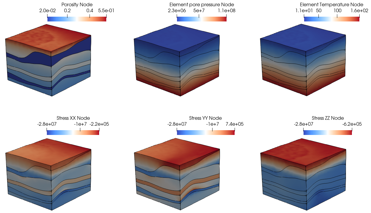
In the figure below there is the distribution of porosity, pore pressure, temperature and stresses after the initialization stages (simulation time 6).

Distribution of stresses, porosity, pore pressure and temperature at the end of initialization
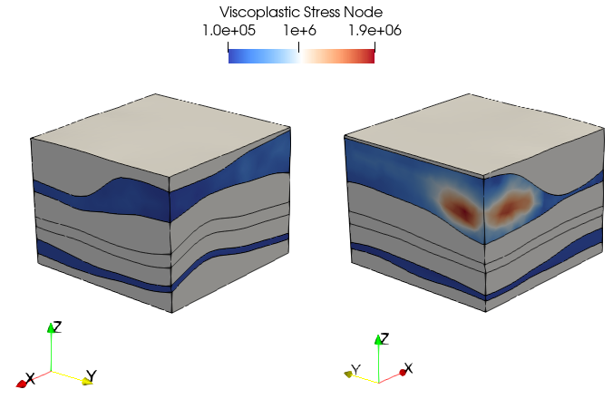
Below is a picture of the viscoplastic stress in salt after initialisation (the viscoplastic stress is the deviatoric stress above the yield stress for creep). As can be seen in most of the salt domain the stress is close to the yield value as the initialisation with viscosity in dKa units facilitated stress relaxation with creep. However due to the geometric features, the interaction of salt with the surrounding formations and the coarse mesh used in this example, achieving a stress state below the creep yield stress within salt in all the domain has not been possible.

Viscoplastic Stress at the end of initialisation (t = 6)
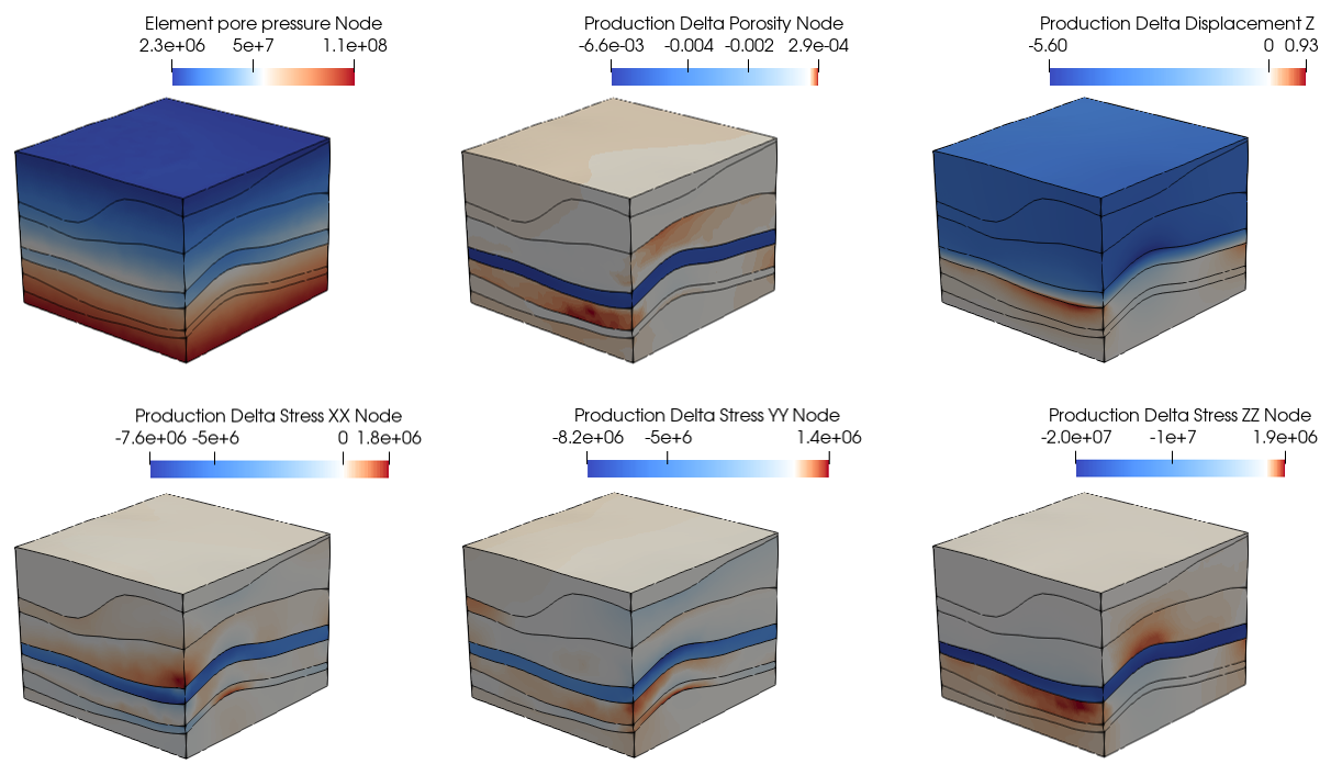
In the figures below it is shown the distribution of pore pressure after the production stages together with the change in vertical displacement, porosity and stresses. It is recalled that the imposed change in pore pressure distribution after the two years of production has been an homogeneous drop of 20·106 Pa across the reservoir while the pore pressure in the remaining formations remains unchanged. It should be noted that such homogeneous drop in pore pressure across the reservoir is not representative of production scenarios where production and injection wells usually perturb the pore pressure field in an inhomogeneous manner. Furthermore the geometrical features of the reservoir also would play a role in non-homogeneous pore pressure distribution. However the current set up was chosen for the sake of simplicity to enable demonstration of the MEM workflow.
As can be seen the pore pressure drop in the reservoir has led to an increase in compressional stresses in the reservoir resulting in porosity decrease due to compaction. Consequently there is a downward trend in displacements for formations above the reservoir. It can be seen that the maximum vertical stress change occurred within the reservoir and its magnitude is consistent with the prescribed drop in pore pressure.

Distribution of pore pressure and change in porosity, vertical displacement and stresses after two years of production. The colour scale for plots showing change in variables has been set so that the 0 (no change) is shown in white, negative changes are shown in blue and positive changes in red.
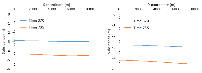
The subsidence after every production year output in the two history section line sets is shown below. As can be seen in both profiles the subsidence increases with production due to the larger drop in pore pressure. In both subsidence profiles the maximum subsidence is observed above the reservoir anticline crest, where the two section lines intersect.

Subsidence results monitored by the two history section line sets. The dotted line indicate the coordinates where the two section lines cross (approximately above the anticline crest).
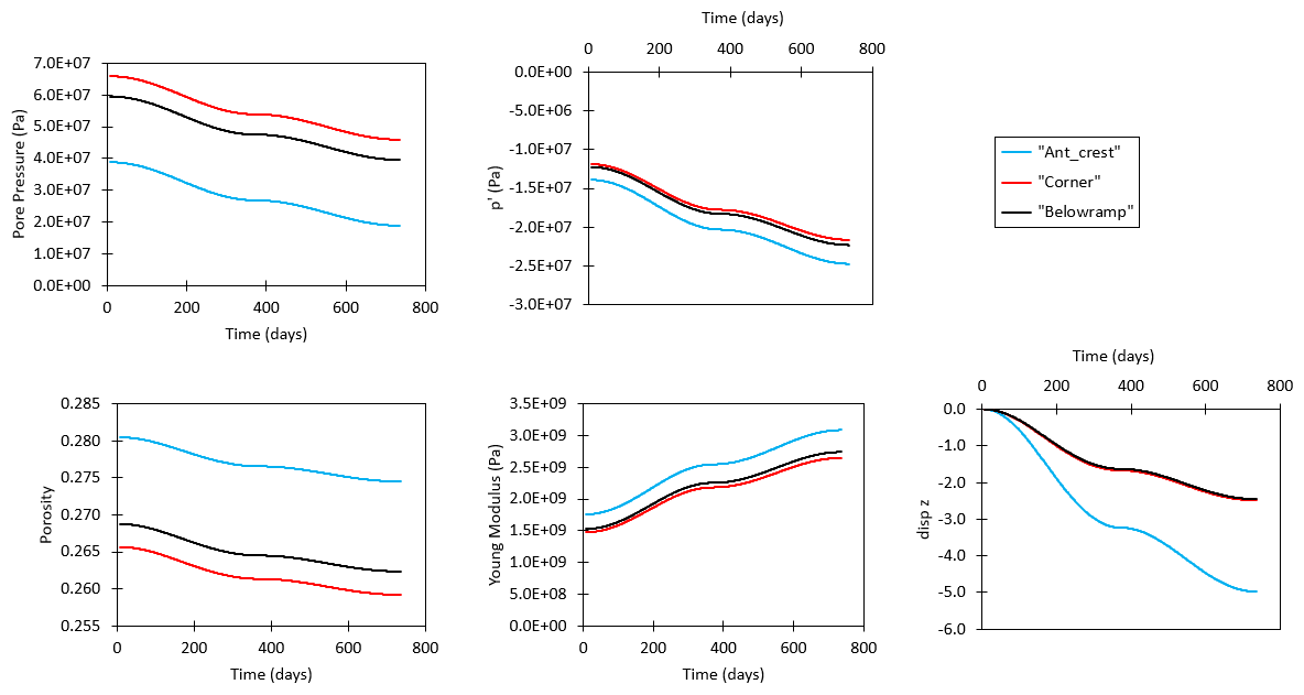
In the figures below the history results for the three points monitored during production within the reservoir are shown. In all points can be seen that as pore pressure drops, compressional effective mean stress increases (becomes more negative) leading to a decrease in porosity, an increase in Young's modulus due the poroelasticity and a downward displacement (subsidence).

History point results for the three points located within the reservoir.
|

