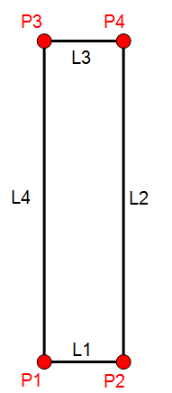
The objective is to simulate the consolidation of a 50m thick column of soil due to a sudden change in the drainage condition at the top surface.   In the initial configuration the soil is fully saturated with an initial pore pressure of 1.0 MPa with no flow allowed through any boundary.  Gravity is neglected, allowing comparison with a classical analytical solution.  The effective stress is zero so that the total mean stress in the column is 1.0 MPa.  Equilibrium in the initial configuration is achieved by applying a 1.0 MPa mechanical stress to the top boundary of the model.  At time t=0 the boundary condition of the top surface is changed to allow free drainage, i.e. pore presssure (pf) = 0, resulting in a gradual dissipation of pore pressure in the model.

The model is analysed in uniaxial strain conditions; i.e. the vertical sides of the model are constrained in the horizontal direction, and the base of the model is constrained in the vertical direction. The column is discretised by a structured mesh of 40 linear quadrilateral (QPM4) elements.

Material Properties

The material corresponding to "HM_001_elastic" has the following mechanical properties :

The additional material parameters related to the porous flow field are:

Notes:

1The simulation uses isotropic permeability.  In general, however, soils exhibit transverse isotropic flow with the horizontal permeability often between 5 to 100 times larger than the vertical permeability.  In this case orthotropic permeability may be defined via Permeability_x, Permeability_y and Permeability_z. Furthermore, permeability is dependent on the current porosity, so that in applications where significant compaction is used permeability is defined as a function of porosity.  This may be either isotropic via Permeability_vs_porosity or orthotropic via Permeability_x_vs_porosity, Permeability_y_vs_porosity and Permeability_z_vs_porosity.

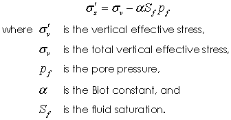
2The Biot constant (Biot_constant) defines the contribution of the pore pressure to the total stress via the effective stress relationship

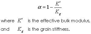
The Biot constant may either be user defined (as in this case) or may be computed automatically via the relationship

3The material is specified as fully saturated ( Fluid_saturation = 1.0).

4The material is saturated with fluid name "Water".

Fluid Properties

The properties of the pore fluid must be specified.  The principal parameters are:

The  data file for the project is : HM_001\Data\hm_001_Case1.dat.   The basic data includes:

1Units defining stress in "MPa", length in "m", time in "years" and temperature in "Celsius".

2Geometry_set data defining model boundaries and domain.

3Mesh control (Mesh_control_data) and structured mesh generation data (Structured_mesh_data and Structured_line_set) defining a uniform mesh with 40 elements in the vertical direction.

4A single group which is assigned the "hm_002_elastic" material properties defined using Group_data and Group_control_data data structures.  The Porous_flow_type = 4 i.e. a coupled geomechanical/porous flow..

5Material properties (Material_data) for "hm001_elastic".

6Fluid properties (Fluid_properties) for water.

7Stratigraphy_definition and Stratigraphy_horizon to define the stratigraphy unit and top surface. Stratigraphy_surface_load to define the applied mechanical stress of 1.0 MPa and a prescribed pore pressure condition (Pore_pressure_flag set to 1) on the top surface.

8Geostatic_data defining initial pore pressure of 1.0 MPa for the model domain.

9Support_data defining geomechanical fixity constraints: base fixed vertically and sides fixed horizontally.

10Damping_global_data defining the use of combined damping models (percentage damping of 2%, i.e. 0.02 and bulk viscosity damping with constant of 0.5) to aid the numerical stability of the column model.

11Point history (History_point) data:

(a)   Set 1: Output of stress and pore pressure at the base of the column every 16 porous flow increments.

(b)  Set 2: Output of pore pressure at 21 points evenly distributed throughout the depth of the column every 16 porous flow increments.

12Solution control data via coupling control data (Couple_control_data) and geomechanical/porous flow control data (Porous_flow_control_data and Control_data)  (see later).

The Group_control_data structure defines the active groups in each field.   Generally all groups are active in all fields.

The Couple_control_data data structure defines the active fields for the analysis and additional data to control the coupling process.  The data structure is only required if more than one field is active.  The majority of the data may be assigned default values.  For coupled hydro-mechanical simulations the default coupling scheme is:

1Fixed Stress algorithm

2Incremental staggered solution strategy

3Data exported from porous flow field: pore pressure and saturation

4Data exported from geomechanical field: coordinates, porosity

Coupling of the geomechanical and porous flow fields is achieved by treating the geomechanical field as an incremental analysis with the time step length corresponding to the time step of the porous flow field; i.e.

1A single porous flow step is performed for every coupling step.  

2The geomechanical field is solved using an "Incremental" control option where multiple time steps are performed in each increment to achieve the explicit solution (dynamic relaxation) of the geomechanical field.

This is necessary as the geomechanical and porous flow fields are "strongly coupled" due to the dependence of pore pressure on the volumetric strain rate.

The data controlling the solution strategy is specified via the Control_data (Geomechanical field) and Porous_flow_control_data (porous flow field) data structures.

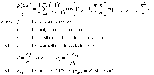
The result files for the project are in directory: HM_001\Results.  The high definition history file results are displayed graphically in the excel file 00_hm_001.xlsx.   The analytical solution is given by

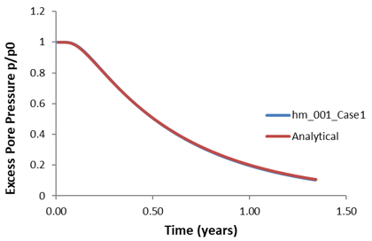
Comparison of the predicted pore pressure evolution at the base of the column with the analytical solution shows an almost exact match.

Pore Pressure Evolution at the Base of the Column Compared to Analytical Solution

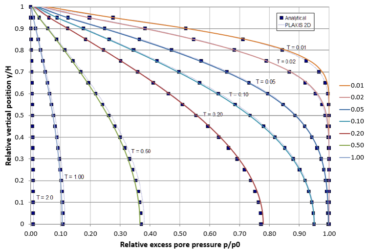
Comparison of the predicted spatial distribution of pore pressure at different normalised times show very good correlation with the analytical solution.

Spatial Distribution of Pore Pressure Compared to Analytical Solution

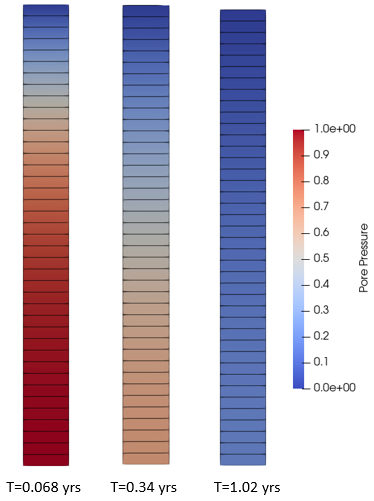
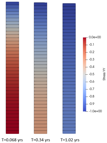
The contour plots of pore pressure and effective vertical stress below shows the gradual dissipation of pore pressure and increase of effective vertical stress with time (the total stress is constant (1.0 MPa) throughout the column).

Contour Plots of Pore Pressure and Effective Vertical Stress-YY at Various Times