For the present tutorial example it is recommended to undertake the following example beforehand:
1MEM_001 Case01 Base Case.
The present case demonstrates the set up of a coupled hydro-mechanical Material Earth Model (MEM) simulation using ParaGeo. This example is similar to Case01 but with the addition of fluid flow which is coupled to the geomechanical analysis and the depletion of the reservoir layer from producer well 3 is modelled via well element definition data structure Well_element using prescribed surface (pore) pressure loading. Initialization is performed in several stages followed by a combined drawdown/depletion stage. The initial values for porosity and pore pressure are defined at an elemental and nodal level, respectively, via Spatial_grid data structures. High perm contact fluid flow is considered at the fault for this example.
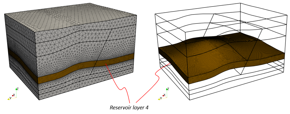
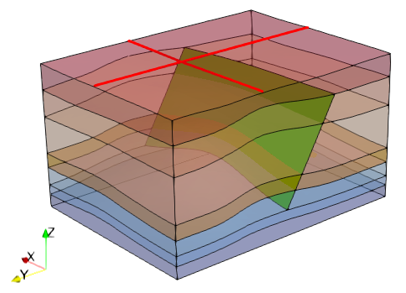
In order to model the fluid flow more accurately, the reservoir layer 4 is discretised with a finer mesh (4 - 7 elements through the layer thickness) than the rest of the formation layers as shown below. Note that the simulation run completes in 1.6 hrs on a 3.6 GHz AMD processor machine.

Finer mesh discretisation in reservoir layer 4.
The data files for the project are in: MEM_001\Case03\Data. The data comprises:
1.geostatic.set: Settings file with pre-defined Geostatic_control_data sets that can be read from the main problem data file. Generally this file is stored in the PARAGEOHOME directory (directory of ParaGeo executable) and is provided here for reference. Note that if a copy of the file is also stored in the simulation directory this will take precedence over the copy stored in PARAGEOHOME directory.
2.MEM_001_Case03a.dat: Main problem data file.
3.MEM_001_Case03_Fine_mesh.geo: Geometry and mesh for the problem with finer mesh discretisation of the reservoir layer 4.
4.MEM_001_Case03.geometry: Data file with definition of geometry sets and groups for the problem including the active groups in the porous flow field and fault contact names.
5.MEM_001_Case03a.contact: Data file with definition of contact, fault and fluid flow contact data for the problem.
6.MEM_001_Case03.mat: Material file including Material_data with permeabilities for all lithologies and Fluid_properties.
7.MEM_001_Case03_Porosity.spat: File containing a Spatial_grid with the initial element porosity values for all formations.
8.MEM_001_Case03_node_PP_Initial.spat: File containing a Spatial_grid with the initial nodal pore pressure values for all formations.
Data set up required to run a faulted MEM hydro-mechanical coupled simulation
In the main, the coupled hydro-mechanical modelling strategy differs from the geomechanical modelling for the faulted anticline in the following aspects:
1Definition of the active groups in the porous flow field in Group_control_data, set Porous_flow_type 4 and define names for the group fault contacts in Group_data (.geometry). 2Definition of material permeabilities in Material_data and fluid flow properties in Fluid_properties (.mat). Grain stiffness, Biot's constant, fluid stiffness and fluid viscosity must also be defined for the flow field although these have already previously been defined in the geomechanical model Case01. 3Contact_flow_flag 1 in Contact_global and definition of fluid flow normal and tangential contact properties in Contact_property (.contact). 4Spatial_grid data defining the initial pore pressures at the nodal level (.spat). 5Definition of Spatial_boundary data for the initial nodal pore pressures via spatial grids (.dat). 6Pore_pressure_flag 1 in Stratigraphy_surface_load (.dat). 7Water_level_data defining the water table level (.dat). 8Well_definition data defining the well loading and status of the specified well points (.dat). 9Definition of Couple_control_data to define the active fields (geomechanical and porous flow) and type of coupling control (.dat). 10Definition of Solver_control to define the implicit solver type to use (.dat). 11Geomechanical/Porous flow solution control Control_data with Solution_algorithm 4, definition of coupling step size via Initial_time_increment and definition of mechanical steps for each coupling step via Target_number_time_steps (.dat).
|
The different simulation stages and the operations performed are described below.
Stage 1: Elastic Gravity Initialization
•Gravity is ramped up during the duration of the stage.
•Initial porosities for the formations are defined via a spatial grid with element values.
•Materials are kept elastic.
•Contact is kept elastic.
•Horizontal stress increases as a function of vertical stress and Poisson's ratio.
•Initial pore pressure distribution is defined via a spatial grid with element values.
•Initial temperature distribution is defined according to a surface temperature and a temperature gradient.
Stage 2: Tectonic Displacement
•A tectonic displacement load is applied in order to obtain the in-situ horizontal stress.
•Materials are kept elastic.
•Contact is kept elastic.
Stage 3: Contact Release
•Materials are kept elastic.
•Contact model is switched from "Elastic" to "Standard".
•Final stresses at the end of the previous stage are saved and ramped up from zero during the present stage.
•Pore pressure is ramped up from zero.
•Displacement on geometry is reinitialized to its original state at the beginning of the stage.
Stage 4: Constitutive Release
•Constitutive models are switched from "Elastic" to "Standard".
•Final stresses at the end of the previous stage are saved and ramped up from zero during the present stage.
•Pore pressure is ramped up from zero.
•Displacement on geometry is reinitialized to its original state at the beginning of the stage and displacement values are reinitialized at the end of the stage.
Stage 5: Drawdown/Depletion - Start of Flow
•Producer well 3 comes online in this stage with a prescribed well surface pressure of 20·106 Pa which is linearly ramped down to 0 Pa over a 1 day time period via Well_definition data structure and corresponding Time_curve_data. Note that this surface pressure value is defined in line with the initial overpressure of 20 MPa in the reservoir (formation04) layer which was previously defined via spatial grid nodal pore pressures. This surface pressure is then subsequently depleted down to reservoir pressure (i.e. zero overpressure) over a 1 day time period. Note that the initial pore pressure in the whole reservoir layer is in the range 34·106 - 69·106 Pa with pressures in the range 47·106 - 51·106 Pa around the producer well 3 "open" locations.
Stage 6: Drawdown/Depletion - Flow
•The zero well surface pressure in producer well 3 is maintained over a 100 day time period.
Descriptions of the data file are provided in the following sections:
•"Model Definition Data" - describes the data defining the model which is not related to initialization or depletion (e.g. geometry, mesh, groups, etc).
•"Well Element Definition Data" - describes the data related to the producer wells.
•"Additional Data Output" - describes the history output data and reference set data.
• Subsequently the data related to each of the stages is described.
Model Definition Data
Here the data defining the model which is not related to initialization or depletion is described. Note that the data may not be described in the same order as it appears in the data file.
Geometry and Mesh
The mesh for the model was generated using Gmsh and exported to Abaqus format. Then the Abaqus --> ParaGeo conversion was used to generate the geometry stored in the MEM_001_Case03_Fine_mesh.geo file.
Data File (.dat)
|
|
* Geometry_data
File_name MEM_001_Case03_Fine_mesh.geo
File_format hdf
* Include
Filename MEM_001_Case03.geometry
|
1.The geometry and mesh for the model is read from the .geo file using the Geometry_data structure.
2.An Include data structure is used to incorporate to the main problem data file the data defined in the .geometry file which contains data for the groups and geometry sets. |
Data File (.geometry)
|
|
* Geometry_set NUM=1
Name "Formation02_top"
Set_type "Abaqus NSET"
Surfaces IDM=3
4 5 10
* Geometry_set NUM=2
Name "Base"
Set_type "Abaqus NSET"
Surfaces IDM=2
29 30
(...)
* Geometry_set NUM=20
Name "Formation07"
Set_type "Group"
Volumes IDM=2
3 10
(...)
* Geometry_set NUM=33
Name "Fault_hgw"
Surfaces IDM=4
83 84 85 86
|
1.The .geometry file contains Geometry_set data structures defining model boundaries, fault contact surfaces, stratigraphy horizons and groups. |
Group data
Data File (.geometry)
|
|
* Group_control_data
Group_numbers IDM=7
1 2 3 4 5 6 7
Active_geomechanical_groups IDM=7
1 1 1 1 1 1 1
Active_porous_flow_groups IDM=7
1 1 1 1 1 1 1
* Group_data NUM=1
Group_name "Formation01"
Element_type "Tet4v"
Material_name "Shale_F01"
Porous_flow_type 4
Geometry_set "Formation01"
Contact_property_name "Fault_shale"
(...)
* Group_data NUM=4
Group_name "Formation04"
Element_type "Tet4v"
Material_name "Reservoir"
Porous_flow_type 4
Geometry_set "Formation04"
Contact_property_name "Fault_sand"
(...)
|
1.A Group_data data structure is defined for each of the seven formations.
2.Group_control_data is used to define geomechanical and porous fields active for the seven formations.
3.Element_type is set to TET4V (4 node 3D tetrahedral elements with average volume formulation) and each formation is assigned the appropriate material data (which is defined in the included .mat file).
4.Porous_flow_type is set to 4 (coupled geomechanical/porous flow analysis with prescribed pore pressure).
5.The Geometry_set defining the volumes for the groups are specified.
6.Material_name containing the material properties (read from .mat file) for each formation is assigned.
7.Contact_property_name containing the fault properties (read from .contact file). |
Materials
The materials are defined in a separate file named MEM_001_Case03.mat which is included in the main data file using the command Include. The properties for the different lithologies are defined so that:
•Reservoir (Formation04) is poroelastic. •Shale formations are elastic. Deeper shale formations have higher Young modulus values than shallower shale formations with values ranging from 1000·106 Pa to 2500·106 Pa. •All formation layers are assigned permeability values. •A single Fluid_properties data structure defines the fluid properties for water applicable to all formations.
Data File (.mat)
|
|
* Material_data
Material_name "Shale_F07"
Grain_stiffness 20000E6
Grain_density 2650.00
Porosity_model_type 1
Porosity 0.30
Elastic_model_type 1
Elastic_properties IDM=2
1000.0E6
0.35
Singlephase_fluid_name "Water"
Permeability 1E-18
* Material_data
Material_name "Reservoir"
Grain_stiffness 20000E6
Grain_density 2650.00
Porosity_model_type 1
Porosity 0.35
Elastic_model_type 1
Elastic_properties IDM=2
2000.0E6
0.20
Porous_elasticity_type 1
Porous_elastic_properties IDM=2
10.0E+6
0.015
Singlephase_fluid_name "Water"
Permeability 1E-12
|
1.Only one shale lithology Material_data is shown here as the different shales only differ in the Young's modulus value which is: ▪Shale_F01: 2500·106 Pa ▪Shale_F02: 2300·106 Pa ▪Shale_F03: 2000·106 Pa ▪Shale_F05: 1700·106 Pa ▪Shale_F06: 1500·106 Pa ▪Shale_F07: 1000·106 Pa
2.The Porosity value (reference porosity) in this case is a dummy parameter as it will be overwritten by values prescribed using the porosity spatial grid data in MEM_001_Case03_Porosity.spat which is included in the main data file using the command Include.
3.Reservoir material is defined poroelasticity data.
4.The shale layers are assigned permeability of 1E-18 m2 (1μD) and the reservoir sand layer a permeability of 1E-12 m2 (1D). |
Contact and Fault data
Contact and fault data is defined in a separate file named MEM_001_Case03a.contact which is included in the main data file using the command Include.
Data File (.contact)
|
|
* Contact_global
Included_contact_sets IDM=1
"All"
Contact_flow_flag 1
* Contact_set NUM=1
Name "All"
Contact_surfaces IDM=2
"Fault_ftw"
"Fault_hgw"
Global_update_frequency 1000
Property_name "Fault_sand"
Buffer_factor 5.0
Print_search 1
* Contact_property NUM=1
Name "Fault_sand"
Compression_model 1
Compression_properties IDM=1
10000.0E6
Tangential_model 2
Tangential_properties IDM=2
10000.0E6
0.2
Flow_model_normal 11
Flow_properties_normal IDM=2
1.157E-14
1.157E-14
Flow_model_tangential 1
Flow_properties_tangential IDM=1
1.157E-11
* Contact_property NUM=2
Name "Fault_shale"
Compression_model 1
Compression_properties IDM=1
10000.0E6
Tangential_model 2
Tangential_properties IDM=2
10000.0E6
0.2
Flow_model_normal 11
Flow_properties_normal IDM=2
1.157E-17
1.157E-17
Flow_model_tangential 1
Flow_properties_tangential IDM=1
1.157E-17
|
1.The data encompasses one Contact_global, one Contact_set, two Contact_surface, two Contact_property and one Fault_set data structures.
2.The Contact_global is defined so that: a.The contact set named "All" is active in the simulation. b.Contact_flow_flag = 1 in order to consider flow contact in the simulation, otherwise even though flow contact properties are specified, the fault would be considered impervious (no flow).
3.The Contact_set is defined so that: a.Hanging wall and Footwall fault contact surfaces are included. b.A global contact search is performed every 1000 mech steps. c.The default contact property assigned to the contact surfaces in the set is named "Fault_sand". d.The buffer factor is set to 5.0 (recommended value). e.The contact search is printed into the .res file.
4.Contact_property for "Fault_sand" is defined with: a.Linear elastic compression contact model with a normal penalty of 10000·106 Pa. b.Coulomb tangential friction contact model with a tangential penalty of 10000·106 Pa and a friction coefficient of 0.2. c.The Flow_model_normal is set to 11 (constant intrinsic permeability). d.In Flow_properties_normal the intrinsic permeabilities for the fracture and the filter cake (fault gouge) are both defined as 1.157·10-14 m2. e.The Flow_model_tangential is set to 11 (constant intrinsic permeability). f.In Flow_properties_tangential the intrinsic permeability is set to 1.157·10-11 m2.
5.Contact_property for "Fault_shale" has same properties as "Fault_sand" except the intrinsic permeabilities for the normal and tangential flow are much lower at 1.157·10-17 m2.
|
Stratigraphy data and Water level data
For MEM applications, definition of the complete stratigraphy is not required but only definition of the top surface. This enables to perform geostatic initialization and any depth-based calculation (e.g. output of element depth variable to plot file, definition of initial temperature as a function of depth). The water level used to define the initial pore pressure applied to the model via spatial grids is also defined via Water_level_data. This will add the load corresponding to the water table level above the top surface.
Data File (.dat)
|
|
* Stratigraphy_definition
Top_surface_horizon "Top"
* Stratigraphy_horizon NUM=1
Name "Top"
Geometry_set "Formation07_top"
* Stratigraphy_surface_load
Applied_stress 0.5E6
Time_curve_stress "Step_scurve"
Pore_pressure_flag 1
* Stratigraphy_smoothing
Active_flag -1
* Water_level_data NUM=1
Water_level 6200
|
1.Stratigraphy_definition and Stratigraphy_horizon are used to identify the top surface (defined by the geometry set "Formation07_top").
2.Stratigraphy_surface_load defines the boundary conditions at the top surface: a.A mechanical stress load of 0.5·106 Pa is applied to the top surface to potentially improve stability by helping to prevent positive stresses developing on the top surface. The load is ramped up following an S-shape function over the duration of the simulation stage ("Step_scurve"). b.Pore_pressure_flag set to 1 indicates that the pore pressure at the top surface horizon is prescribed (this is default in coupled problems).
3.Stratigraphy smoothing is off during the simulation (Active_flag set to -1).
4.Water_level_data defines the water table level at 6200m which is used to define the initial pore pressure spatial grid data for the model. |
Support data
Data File (.dat)
|
|
* Support_data
Displacement_codes IDM=3 JDM=4
1 0 0
0 1 0
0 0 1
1 1 1
Displacement_code_geom_set IDM=5
"East"
"West"
"North"
"South"
"Base"
Displacement_code_geom_ass IDM=5
1 1 2 2 3
|
1.Displacements are constrained in the normal direction for the Base and side boundaries.
|
|
Well Element Definition Data
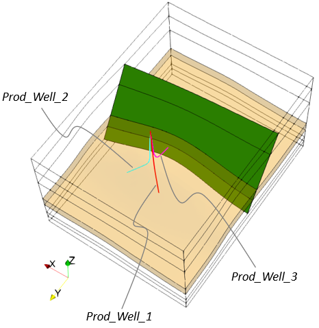
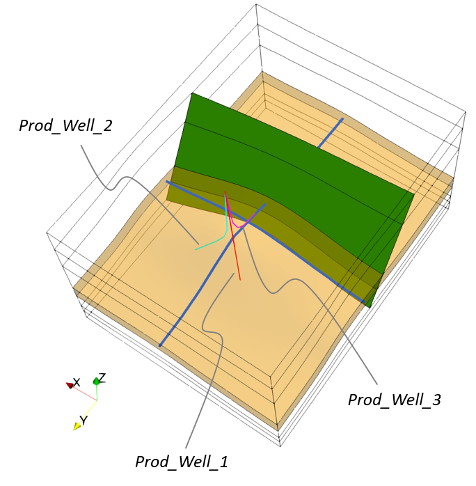
Data definition for three producer wells are described here, however, only producer well #3 is utilised for production in this example. Note that producer well #3 will not come online until stage 5, however, it is recommended that the wells are defined in stage 1 with the well points 'shut' and then updated to 'open' when they come online in the later stages. This enables the user to visualize and track the wells throughout the simulation.
Note that when the well loading is defined with Surface_pressure, care must be taken to ensure that when the well comes online, the value of the pressure defined is in line with initial conditions.
Data File (.dat, .set)
|
|
* Well_definition NUM=1
Name "Prod_Well_1"
Well_type "Producer"
Well_path IDM=3 JDM=39
4500 6400 5947
4492 6408 5848
4483 6417 5748
....
3649 7251 2889
3582 7318 2846
3500 7400 2800
Well_radius 1.00
Status_distribution IDM=39
"casing"
"shut"
"shut"
....
"shut"
"shut"
"shut"
Surface_pressure 1.0
Time_curve 200
Singlephase_fluid_name "Water"
Flow_model 3
Output_level 1
History_summ_frequency 1
* Well_definition NUM=2
Name "Prod_Well_2"
Well_type "Producer"
Well_path IDM=3 JDM=39
4500 6400 5947
4504 6404 5847
4509 6409 5747
....
5211 7111 2828
5276 7176 2784
5400 7300 2700
Well_radius 1.00
Status_distribution IDM=39
"casing"
"shut"
"shut"
....
"shut"
"shut"
"shut"
Surface_pressure 1.0
Time_curve 200
Singlephase_fluid_name "Water"
Flow_model 3
Output_level 1
History_summ_frequency 1
* Well_definition NUM=3
Name "Prod_Well_3"
Well_type "Producer"
Well_path IDM=3 JDM=38
4500 6400 5947
4500 6395 5847
4500 6390 5747
....
4500 5524 2999
4500 5425 2968
4500 5327 2937
4500 5200 2900
Well_radius 1.00
Status_distribution IDM=38
"casing"
"shut"
"shut"
....
"shut"
"shut"
"shut"
Surface_pressure 1.0
Time_curve 200
Singlephase_fluid_name "Water"
Flow_model 3
Output_level 1
History_summ_frequency 1
* Time_curve_data NUM=200
! --------------------------------------
Name "Depletion"
Curve_type 1
Time_curve IDM=3
4.0 5.0 105.0
Load_factor IDM=3
2.0E+07 0.0 0.0
|
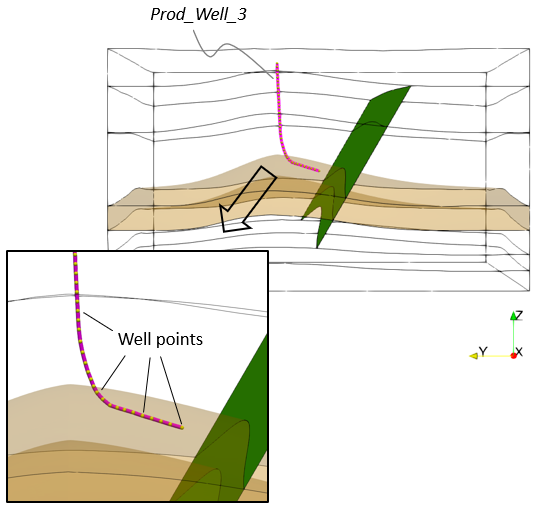
1.Well_definition data structure is defined for the three production wells, however, the following descriptions will be directed at well #3: a.Name - The production well is named "Prod_Well_3". b.Well_type - Defines the well type as "Producer" well. This keyword is required in conjunction with Surface_pressure well loading. It is not required if Injection_rate or Production_rate is defined. c.Well_path - Defines the x, y and z coordinates of the 38 well points from top to bottom. d.Well_radius - A constant well radius of 1.0 m is defined. e.Status_distribution - The status distribution for all well points is defined as "casing" (no leak off) at the top and "shut" (no leak off) for all other well points at the start of the simulation. Note that the "shut" status will be changed to "open" in the reservoir section of the well (i.e. formation04) during the depletion stage. f.Surface_pressure - A surface pressure of 1.0 Pa is defined in conjunction with the Time_curve_data 200 to give a well surface pore pressure of 20 MPa (i.e. over-pressure of 20 MPa in the reservoir well points in line with the initial pore pressures defined) at the start of depletion time=4. g.Singlephase_fluid_name - The well fluid is defined as "Water", same as the pore fluid in the formation. h.Flow_model - The well flow model is defined as hydrostatic prescribed based on surface pressure (default). i.Output_level - The level of output detail of well information (pressure/flow rates) in the .res file is defined as 1 (standard). j.History_summ_frequency set to 1 defines the output of well history data every step. The name of the well will be appended to the file name, e.g. "MEM_001_Case03a_Prod_well_3_summ.hdh".
2.Time_curve_data 200 defines the time curve associated with the well loading, in this case, the Surface_pressure which is applied as a linear ramp over 1 day.

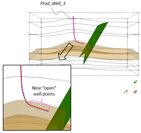
Location of three producer wells

Well definition for producer well #3
|
|
Additional Data Output
The data used to request additional plot file output defined within Control_data is described here. The additional data output includes:
1.One History_global set to output the evolution of global energies in the geomechanical field. 2.One History_point set with one point at each formation for monitoring initialization. 3.Two History_point sets for monitoring changes in the reservoir (Formation04) and seal (Formation05) during depletion. 4.Two history line outputs (History_section_line) to output vertical displacement profile at the top surface. 5.Two history line outputs (History_section_line) to output element pore pressures in the reservoir (Formation04). 6.Two History_surface to output contact data on the fault. 7.An Output_data data structure defining the data for output (0 - no output, 1 - output) to plot files to help to reduce the size of the results plot files. 8.A Reference_set_data data structure to request output of change in selected variables during depletion.
Initialization Stages
Data File (.dat)
|
|
* History_global
Output_frequency_time 0.02
Mech_global_energy_data IDM=7
"Kinetic" "Elastic" "External" "Inelastic"
"Bulk_visc" "Damping" "Cont_damp"
* History_point NUM=1
Name "Initialization"
Output_frequency_time 0.02
Point_labels IDM=7
"Formation01"
"Formation02"
(...)
"Formation07"
Point_coordinates IDM=3 JDM=7
4500 6400 1000
4500 6400 1900
(...)
4500 6400 5800
Displacements IDM=3
"Disp_x" "Disp_y" "Disp_z"
Velocities IDM=3
"Veloc_x" "Veloc_y" "Veloc_z"
(...)
Element_data IDM=2
"Porosity" "Elt_pore"
Elastic_state_variables IDM=1
"Young"
* History_section_line NUM=1
Name "ReservoirY"
Output_frequency_increment -1
Output_formats IDM=1
"psect"
Point_distribution_type 0
Point_distance 100
Path_coordinates IDM=3 JDM=11
4500 0 2089
4500 584 2115
4500 1839 2181
4500 2848 2308
4500 3845 2510
4500 5143 2834
4500 6400 3059
4500 7379 2747
4500 8304 2403
4500 9292 2180
4500 10400 2089
Element_data IDM=1
"Elt_pore"
* History_section_line NUM=2
Name "ReservoirX"
Output_frequency_increment -1
Output_formats IDM=1
"psect"
Point_distribution_type 0
Point_distance 100
Path_coordinates IDM=3 JDM=11
0 5600 2128
1059 5600 2285
2031 5600 2501
2998 5600 2739
3978 5600 2914
4970 5600 2912
5900 5600 2721
6777 5600 2517
7120 5600 2443
7569 5600 2361
8000 5600 2287
Element_data IDM=1
"Elt_pore"
* History_section_line NUM=3
Name "SubsidenceY"
Output_frequency_increment -1
Point_distribution_type 0
Point_distance 100
Path_coordinates IDM=3 JDM=3
4500 10400 5925
4500 6400 5975
4500 0 5930
Displacements IDM=1
"Disp_z"
* History_section_line NUM=4
Name "SubsidenceX"
Output_frequency_increment -1
Point_distribution_type 0
Point_distance 100
Path_coordinates IDM=3 JDM=3
0 6400 5955
4500 6400 5985
8000 6400 5918
Displacements IDM=1
"Disp_z"
* History_surface NUM=4
! ---------------------------------
Name "Fault_hgw"
Geometry_sets IDM=1
"Fault_hgw"
Contact_point_values IDM=5
C_strsnm
C_strsne
C_strstn
C_qprat
C_pslip
Output_frequency_step -1
Output_name_flag 1
Output_topology_flag 1
* History_surface NUM=5
! ---------------------------------
Name "Fault_avg_hgw"
Geometry_sets IDM=1
"Fault_hgw"
Average_values IDM=6
C_strsnm
C_strsne
C_strstn
C_qprat
C_pslip
C_por_pr
Output_frequency_increment 1
Output_name_flag 1
Output_topology_flag 1
|
1.A History_global data structure is used to monitor the evolution of the global energies in the geomechanical field.
2.A History_point data structure is used to monitor the evolution of the specified variables during initialization.
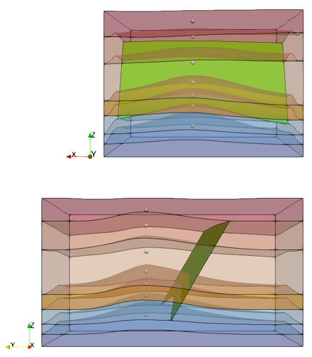
3.There is one point defined for each of the formations which are arbitrarily located at the X and Y coordinates corresponding to the anticline crest.

Location of history points for monitoring initialization stages
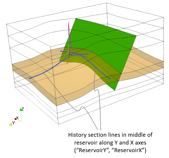
4.Two History_section_line data structures are defined to monitor the depletion profile along the reservoir at the end of each simulation stage. To this end, element pore pressures are output every 100m in the middle of the reservoir along the X and Y axes directions, crossing at point (x,y) = (4500, 5600) which is the location of the producer well 3 in the reservoir (see image below).
5.The history section line name will be appended to the file name, e.g. MEM_001_Case03a_ReservoirY_X.psect, where X is the simulation stage number.


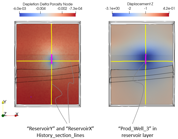
Location of history section lines "ReservoirX" and "ReservoirY"
6.Two History_section_line data structures are defined to output top surface vertical displacement (subsidence) along X and Y axis both crossing point (x, y) = (4500, 6400) located above the anticline crest (see image below). Note that: a.The data is defined at the last initialization stage so that the initial displacement before depletion is also output allowing to calculate the true increments due to depletion. b.Output is performed at the end of each stage (Output_frequency_increment set to -1). c.Output is performed every 100 m (Point_distance set to 100).

Location of the history section lines "SubsidenceX" and "SubsidenceY"
7.Two History_surface data structures are defined in order to output the following contact data variables for the Fault_hgw contact surface, one history for output at the contact points and another history for the average value output. The history output at the contact points will be at the end of each stage (Output_frequency_step set to -1) and the average contact history output will be every increment: a.C_strsnm: Contact total stress normal b.C_strsne: Contact effective stress normal c.C_strstn: Contact tangential stress d.C_qprat: Contact effective stress ratio e.C_pslip: Contact plastic slip f.C_pore_pr: Contact pore pressure
8.The name of the contact surface (Fault_hgw / Fault_avg_hgw) will be appended to the file name: a.For the history output at the contact points, the output file names will be MEM_001_Case03a_Fault_hgw_X.cfs where X is the output number (stage number for the present case as output will only be performed at the end of each stage). b.For the average contact history output, the output file name will be MEM_001_Case03a_Fault_avg_hgw.hdh
9.Output_topology_flag set to 1 is defined to request output of a file describing the contact surface topology. The file will be named MEM_001_Case03a_Fault_hgw.topo / MEM_001_Case03a_Fault_avg_hgw.topo
|
Output data
Data File (.dat)
|
|
* Output_data
Name "MEM_output"
Nodal_output_flags IDM=7
1 1 1 1 0 0 0
Element_output_flags IDM=13
1 0 1 1 0 1 1 1 0 0 0 1 0
State_variable_flags IDM=13
1 0 1 0 0 0 0 0 0 0 1 0 0
|
1.An Output_data data structure defining the data for output (0 - no output, 1 - output) to plot files is specified. This can help to reduce the size of the results plot files. a.Nodal data for output include Displacements, Velocity, Pore pressure and Temperature. b.Element data for output include Stress, State variables, Stress invariants, Element variables, Porous flow velocity, Porous flow gradient and Pore pressure (element). c.State variables data for output include Elastic, Plastic and Porous flow state variables.
|
Drawdown/Depletion Flow Stages
Data File (.dat)
|
|
* Reference_set_data NUM=1
Name "Depletion"
Output_change 1
Groups IDM=7
"Formation01"
"Formation02"
(...)
"Formation07"
Nodal_variables IDM=2
"Disp" "Pore_nod"
Element_variables IDM=6
"Porosity" "Effmean" "Vonmises"
"Strs_xx" "Strs_yy" "Strs_zz"
* History_point NUM=1
Active_flag -1
* History_point NUM=2
Name "Reservoir"
Group_name "Formation04"
Output_frequency_increment 1
(...)
* History_point NUM=3
Name "Seal"
Group_name "Formation05"
Output_frequency_increment 1
(...)
|
1.A Reference_set_data is defined at the start of the flow stage so that the change in the specified variables is output to the plot file. Because the data is named "Depletion" the output variables will be named according to the following format: "Depletion Delta Porosity".
2.The history output for the history point set number 1 (defined to monitor initialization) is requested to be deactivated and removed during the depletions stages via Active_flag set to -1. This is done to avoid too many outputs resulting from the depletion stage (note that Output_frequency_time for history point set was defined as 0.02 time units and the depletion stage have a total duration of 105 days).
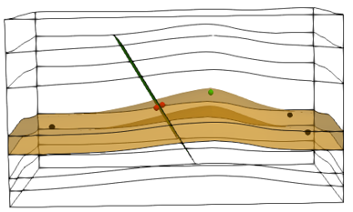
3.Two History_point set data structures are defined to monitor evolution of selected variables during depletion. The objective of each History_point set is to monitor evolution of specified properties at six locations in the reservoir and the overlaying seal. These locations are the anticline crest (green point in the figure below), three downdip locations (black points) and two at both sides of the fault (red points). Points in the seal (not shown) are above those for the reservoir. The results are defined to be output every time increment (Output_frequency_increment set to 1).

Reservoir history points locations to monitor depletion stages.
|
|
Stage 1: Elastic Gravity Initialization Data
Definition of initial Units
In the present case, definition of Units is relevant as it allows gravity to be defined as 9.81 m/s2 and the code will perform the corresponding scaling according to the units chosen.
Data File (.dat)
|
|
* Units
Length "m"
Stress "Pa"
Time "days"
Temperature "Celsius"
Permeability "m^2"
Conductivity "W"
|
1.The Units for the problem are defined.
|
Gravity data
Data File (.dat)
|
|
* Gravity_data
Gravity_constant 9.81
Time_curve "Step_scurve"
|
1.Gravity_data is defined with gravity being applied following an S-shape function over the duration of the simulation stage ("Step_scurve"). |
Geostatic data and definition of initial porosity and pore pressure
The initial porosity and pore pressure distribution for shale and reservoir formations are defined at an element and nodal level, respectively, via a Spatial_grid and prescribed using Geostatic_data. Geostatic_control_data is used to call the initialization options for the current stage which are defined in the geostatic.set file.
Data File (.dat, .set, .spat)
|
|
* Geostatic_control_data
Include_set_name "Gravity"
* Geostatic_control_data
Description "Gravity"
Stress_constitutive_model "Elastic"
Contact_constitutive_model "Elastic"
Stress_initialisation_type "Standard"
Displacement_reinit_flag 0
State_reinit_flag 1
Time_curve "Step_scurve"
* Geostatic_data NUM=1
Name "Initialisation"
Groups IDM=7
"Formation01"
"Formation02"
(...)
"Formation07"
Porosity_spatial_grid "Porosity"
* Include
Filename MEM_001_Case03_Porosity.spat
* Include
Filename MEM_001_Case03_node_PP_Initial.spat
* Spatial_grid
Name "Porosity"
Type "Element"
Element_variables IDM=1
"Porosity"
Element_numbers IDM=448195
1 2 ...
... 448194 448195
Element_values IDM=1 JDM=448195
0.14448
0.14505
(...)
0.33351
* Spatial_grid
Name "Pore_Pressure_Initial"
Type "Nodal"
Nodal_variables IDM=1
"Pore_nod"
Node_numbers IDM=78102
1 2 ...
... 78101 78102
Nodal_values IDM=1 JDM=78102
1.32E+07
1.13E+07
(...)
1.39E+07
* Spatial_boundary NUM=1
Name "Pore Pressure"
Boundary_type "Spatial_grid"
Spatial_grids IDM=1
"Pore_Pressure_Initial"
Prescribed_components IDM=1 JDM=1
4
Time_curve "Step_scurve"
|
1.In Geostatic_control_data the options for the current initialization stage are defined within the geostatic.set file and those are (only data relevant to the current model is discussed): a.The materials will be kept elastic (Stress_constitutive_model set to Elastic) b.The stresses are initialized with gravity (Stress_initialization_type set to Standard) c.Contact will be kept elastic (Contact_constitutive_model set to Elastic) d.No displacement re-initialization will be performed (Displacement_reinit_flag = 0) e.State variable re-initialization is performed after the end of the stage (State_reinit_flag = 1)
2.Geostatic_data is defined in order to use the values defined in the spatial grid named "Porosity" to prescribe the initial porosity.
3.It should be noted that initial porosity values could also be prescribed using a Spatial_state_set and assigning the porosity grid instead of using Geostatic_data. Nonetheless usage of Geostatic_data is generally preferred because in cases involving plastic materials with hardening, the initial plastic volumetric strain should be evaluated from the initial porosity value and the reference porosity in order to obtain an appropriate initial value for pre-consolidation pressure (this procedure is only invoked when using Geostatic_data).
4.The Spatial_grid defining element porosity and initial nodal pore pressure values are defined in separate files named MEM_001_Case03_Porosity.spat and MEM_001_Case03_node_PP_Initial.spat, respectively, which are included in the main data file by using the data structure Include.
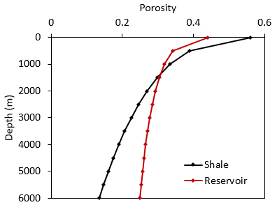
5.MEM_001_Case03_Porosity.spat file contains Spatial_grid "Porosity" data for the element variable "Porosity" for the 448,195 elements of the domain. The element numbers and their corresponding porosity values are specified. The porosity curves used to define the grid are shown in the image below.

Compaction curves used to define the porosity grid
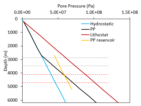
6.MEM_001_Case03_node_PP_Initial.spat contains Spatial_grid "Pore_Pressure_Initial" data for the nodal variable "Pore_node" for the 78,102 nodes of the domain. The node numbers and their corresponding pore pressure values are specified. The pore pressure curves used to define the grid are shown in the image below. The overpressure in the shales start at 2.5 km below mud line and the pore pressure profile follows a trend parallel to the lithostatic whereas the reservoir pore pressure trend is parallel to the hydrostatic gradient with an overpressure of 18 MPa.
7.The Spatial_boundary data structure is defined in order to use the values defined within the "Pore_Pressure_Initial" spatial grid to prescribe the initial pore pressure at nodal basis (Prescribed_components set to 4). Note that the initial pore pressure will be gradually ramped up from zero synchronous to gravity as both are assigned an S-curve over the duration of the simulation stage ("Step_scurve").

Pore pressure distribution with depth defined via the spatial grid
|
Support data
Note that the support data for the stage 1 initialization stage applies to the other initialization stages and does not require to be redefined.
Data File (.dat)
|
|
* Support_data
Displacement_codes IDM=3 JDM=4
1 0 0
0 1 0
0 0 1
1 1 1
Displacement_code_geom_set IDM=5
"East"
"West"
"North"
"South"
"Base"
Displacement_code_geom_ass IDM=5
1 1 2 2 3
|
1.Displacements are constrained in the normal direction for the Base and side boundaries.
|
Temperature Distribution
The initial temperature distribution is defined via a Global_loads and a Spatial_variation_definition.
Data File (.dat)
|
|
* Global_loads NUM=1
Name "Temperature vs. Depth"
Prescribed_temperature IDM=1 JDM=1
1.0
Prescribed_temperature_spatial 1
Pres_temperature_geom_set IDM=1
"All_volumes"
Pres_temperature_geom_ass IDM=1
1
* Spatial_variation_definition NUM=1
Description "Temperature vs. Depth"
Type "Absolute"
Distribution "Depth_dependent"
Variation_assignment 1
* Spatial_variation_values NUM=1
Description "Temp. vs. Depth"
Time 0.0
Values_vs_depth IDM=2 JDM=2
0.0 20960.5
10.0 534.013
* Time_curve_data NUM=1
Name "Temperature"
Time_curve IDM=2
0.0 1.0
Time_factor IDM=2
1.0 1.0
Curve_type 1
* Load_case_control_data
Loadcases IDM=1
1
Active_load_flags IDM=1
2
|
1.A Global_loads data structure is defined to prescribe a spatial distribution of temperature.
2.A single Prescribed_temperature set is defined with its value set to 1.0. Note that this will not be used as the spatial distribution will be used instead.
3.Prescribed_temperature_spatial is assigned Spatial_variation_definition number 1.
4.The prescribed temperature set is assigned to "All_volumes" geometry set (a reserved geometry set generated by the code that encompasses all the volumes in the domain).
5.The Spatial_variation_definition and Spatial_variation_values define the temperature distribution with depth.
6.The temperature is prescribed as an instantaneous load (Global_loads NUM=1 uses the defined Time_curve_data NUM=1). The values are defined according to a surface temperature of 10 ºC and a temperature gradient of 0.025 ºC/m. |
Couple Control Data
Data File (.dat)
|
|
* Couple_control_data
Field_names IDM=2
"Geomechanical"
"Porous_flow"
Volume_strain_coupling "None"
Solution_algorithm "Incremental"
* Solver_control NUM=1
Solver_type "Petsc"
|
1.Couple_control_data data structure defines the active fields (i.e. geomechanical and porous flow) for the analysis and additional data to control the coupling process. The data structure is only required if more than one field is active. The majority of the data may be assigned default values. For coupled hydro-mechanical simulations the default coupling scheme is: a.Volume_strain_coupling set to "None" for the initialization stages. No change in parameters, e.g. pore pressure, displacements, porosities will contribute to the volume strain during the initialization stages. b.Incremental staggered solution strategy.
2.The implicit iterative "Petsc" solver type is adopted to solve for the porous flow field.
|
Solution Control Data for Coupled Geomechanical/Porous Flow
Coupling of the geomechanical and porous flow fields is achieved by treating the geomechanical field as an incremental analysis with the time step length corresponding to the time step of the porous flow field; i.e.
1A single porous flow step is performed in each time step for the coupled problem. 2The geomechanical field is solved using an "Incremental" control option where multiple time steps (iterations) are performed in each increment to achieve the explicit solution (dynamic relaxation) of the geomechanical field. This is necessary as the geomechanical and porous flow fields are "strongly coupled" due to the dependence of pore pressure on the volumetric strain rate.
The data controlling the solution strategy is specified via the Control_data (Geomechanical field) and Porous_flow_control_data (porous flow field) data structures. In this example, and is often the case, the data for the porous flow field can be set using the default values so that only the Control_data data structures are specified.
Data File (.dat)
|
|
* Porous_flow_control_data
Control_title "init"
Solution_algorithm 2
* Control_data
Control_title "init"
Solution_algorithm 4
Duration 1.0
Initial_time_increment 0.02
Target_number_time_steps 200
Output_frequency_plotfile -1
Output_time_plotfile 0.2
Output_frequency_restart -1
Screen_message_frequency 10
|
1.Porous_flow_control_data data structure defines the data specific to the porous flow solution control. a.The Solution_algorithm is set to 2 (nonlinear static) during the four initialization stages.
2.Control_data data structure defines coupled geomechanical/porous flow solution data for the stage. All four initialization stages have identical control data with the exception of the Target_number_time_steps (see below) so that only the present initialization control stage will be described in detail. The key data comprises: a.Solution_algorithm set to 4 (incremental transient algorithm) which allows more iterations in an increment if the solution is not converged. b.Duration is set to 1.0 time units. c.Initial_time_increment is set to 0.02, i.e. coupling time step of 0.02 time units. d.The Target_number_time_steps is set to 200, i.e. 200 mechanical steps per coupling step for the gravity and tectonic stages #1 and #2 and set to 400 for the contact release and constitutive release stages #3 and #4. More geomechanical steps are found to be necessary for this example contact release and constitutive release stages to minimize the influence of dynamics. e.Screen_message_frequency is set to 10, i.e. simulation information will be printed to the command prompt every 10 coupling steps. f.A plot file will be output every 0.2 time units (Output_time_plotfile set to 0.2) and at the end of the stage (Output_frequency_plotfile set to -1). g.A restart file will be output at the end of the stage (Output_frequency_restart set to -1). |
|
Stage 2: Tectonic Displacement
Geostatic Options
Data File (.dat, .set)
|
|
* Geostatic_control_data
Include_set_name "Tectonic"
* Geostatic_control_data
Description "Tectonic"
Stress_constitutive_model "Elastic"
Contact_constitutive_model "Elastic"
Stress_initialisation_type "None"
Displacement_reinit_flag 0
State_reinit_flag 0
Time_curve "Step_constant"
* Spatial_boundary NUM=1
Name "Pore Pressure"
Boundary_type "Spatial_grid"
Spatial_grids IDM=1
"Pore_Pressure_Initial"
Prescribed_components IDM=1 JDM=1
4
Time_curve "Step_constant"
|
1.In the geostatic.set file the Geostatic_control_data options for the current stage are defined which are: a.Materials are kept elastic. b.Stresses are not initialised (values calculated from the previous stage are kept as the initial values). c.No displacement re-initialization nor state variable re-initialization is performed (flags set to 0). d.Because we are not interested in re-initializing the values during this stage, a time curve with constant load factor over the duration of the stage is assigned ("Step_constant").
2.Spatial_boundary needs to be re-specified in order to consider the initial pore pressure values defined by the spatial grid. Because we are not interested in re-initializing the values during this stage (as we do not re-initialize stresses) a time curve with constant load factor over the duration of the stage is assigned ("Step_constant").
|
Tectonic Load
Data File (.dat)
|
|
* Global_loads NUM=2
Name "Tectonic_disp"
Prescribed_displacement IDM=3 JDM=1
0.0 1.0 0.0
Pres_displacement_geom_set IDM=1
"North"
Pres_displacement_geom_ass IDM=1
1
* Time_curve_data NUM=2
Name "Tectonic_disp"
Time_curve IDM=2
1.0 2.0
Time_factor IDM=2
0.0 -25.0
Curve_type 2
* Load_case_control_data
Loadcases IDM=2
1 2
Active_load_flags IDM=2
2 2
|
1.A prescribed contractional displacement of 25 m is applied to the "North" boundary. This is achieved by: a.Defining a Global_loads data structure with a prescribed displacement set with a displacement of 1.0 m in the Y direction. b.Assigning the displacement set to "North" boundary. c.Defining a multiplication factor of -25.0 in the corresponding time curve.
2.The Global_loads number 2 defining the tectonic displacement is defined as active (flag = 2) as well as Global_loads number 1 corresponding to the temperature load.
|
|
Stage 3: Contact Release
Geostatic Options
Data File (.dat, .set)
|
|
* Geostatic_control_data
Include_set_name "Contact_release"
* Geostatic_control_data
Description "Contact_release"
Stress_constitutive_model "Elastic"
Stress_initialisation_type "Standard"
Contact_constitutive_model "Standard"
Displacement_reinit_flag 1
Poroelastic_init_flag 1
State_reinit_flag 1
Time_curve "Step_scurve"
* Spatial_boundary NUM=1
Name "Pore Pressure"
Boundary_type "Spatial_grid"
Spatial_grids IDM=1
"Pore_Pressure_Initial"
Prescribed_components IDM=1 JDM=1
4
Time_curve "Step_scurve"
|
1.In geostatic.set file Geostatic_control_data options for the current stage are defined which are as follows: a.Materials are kept elastic (Stress_constitutive_model set to "Elastic"). b.Stresses are re-initialised (Stress_initialisation_type set to "Standard"). c.Displacement is re-initialized at the beginning of the present simulation stage so that the geometry will go back to the state prior to any compaction and tectonic displacement (Displacement_reinit_flag 1). d.Poroelastic_reinit_flag set to 1 indicates that the stresses at the end of the previous stage are used to evaluate poroelastic constants (i.e. Bulk modulus) otherwise because we are re-initializing stresses the initial bulk modulus may be relatively low leading to development of elastic strains as stress increase during the stage. e.State variable values are re-initialized after the end of the stage (State_reinit_flag set to 1).
2.Spatial_boundary needs to be re-specified in order to consider the initial pore pressure values defined by the spatial grid. An s-shaped time curve is defined so that values are ramped up from 0 over the duration of the stage.
|
Solution Control Data
Data File (.dat, .set)
|
|
* Control_data
Control_title "Release_contact"
...
Target_number_time_steps 400
...
|
1.The Control_data data structure is identical to the first initialization stage with the exception of the Target_number_time_steps which is increased from 200 to 400. More geomechanical steps are found to be necessary for this example's contact release stage in order to minimize the influence of dynamics.
|
|
Stage 4: Constitutive Release
Geostatic Options
Data File (.dat, .set)
|
|
* Geostatic_control_data
Include_set_name "Elastic_release"
* Geostatic_control_data
Description "Elastic_release"
Stress_constitutive_model "Standard"
Stress_initialisation_type "Standard"
Displacement_reinit_flag 3
Poroelastic_init_flag 1
State_reinit_flag 1
Time_curve "Step_scurve"
* Spatial_boundary NUM=1
Name "Pore Pressure"
Boundary_type "Spatial_grid"
Spatial_grids IDM=1
"Pore_Pressure_Initial"
Prescribed_components IDM=1 JDM=1
4
Time_curve "Step_scurve"
|
1.In geostatic.set file Geostatic_control_data options for the current stage are defined which are as follows: a.Materials are using the constitutive properties as defined in Material_data (Stress_constitutive_model set to "Standard"). b.Stresses are re-initialised (Stress_initialisation_type set to "Standard"). c.Displacement on geometry is re-initialized at the beginning of the simulation stage (returning back to the state prior to any compaction) and displacement variable value is set to zero at the end of the present simulation stage (Displacement_reinit_flag 3). d.Poroelastic_reinit_flag set to 1 indicates that the stresses at the end of the previous stage are used to evaluate poroelastic constants (i.e. Bulk modulus) otherwise because we are re-initializing stresses the initial bulk modulus may be relatively low leading to development of elastic strains as stress increase during the present initialization stage. e.State variable values re-initialized at the end of the stage (State_reinit_flag set to 1).
2.Spatial_boundary needs to be re-specified in order to consider the initial pore pressure values defined by the spatial grid. An s-shaped time curve is defined so that values are ramped up from 0 over the duration of the stage. |
Solution Control Data
Data File (.dat, .set)
|
|
* Control_data
Control_title "Release_material"
...
Target_number_time_steps 400
...
|
1.The Control_data data structure is identical to the first initialization stage with the exception of the Target_number_time_steps which is increased from 200 to 400. More geomechanical steps was found to be necessary for this example's constitutive release stage in order to minimize the influence of dynamics.
|
|
Stages 5 and 6: Drawdown/Depletion Flow Stages
Well Definition Data
Producer well 3 comes online in this stage. The well data previously defined in stage 1 still applies and the re-definition of the well data need only consist of the name of the well, the status distribution (and well loading time curve if different from previously defined). In this case, only the status distribution for the nine well points in the reservoir (formation04) layer is changed from "shut" to "open" for producer well 3.
Note that the simulation of depletion is split into two stages - start of flow and flow. Stage 5 - start of flow simulates the 1 day duration with high drawdown rate of 20·106 Pa/day and Stage 6 - flow simulates the remaining 100 days of depletion. Data definition for stages 5 and 6 is similar apart from the control stage whereby smaller coupling time step increments are used for the start of flow.
Data File (.dat, .spat)
|
|
* Well_definition NUM=3
Name "Prod_Well_3"
Status_distribution IDM=38
"casing"
"shut"
"shut"
....
"shut"
"open"
"open"
"open"
"open"
"open"
"open"
"open"
"open"
"open"
|
1.Well_definition #3 data structure is re-defined for the producer well 3 in stage 5 production: a.Status_distribution - The status distributions for the bottom nine "shut" well points in the reservoir layer (formation04) are changed to "open".

Producer well #3 'open' well points in reservoir layer (formation04)
|
Couple Control Data for Flow Stages
Data File (.dat)
|
|
* Couple_control_data
Field_names IDM=2
"Geomechanical"
"Porous_flow"
Volume_strain_coupling "Fixed_stress"
Solution_algorithm "Incremental"
|
1.The Couple_control_data data structure is re-defined for the flow stages such that: a.Volume_strain_coupling set to "Fixed_stress". b.Incremental staggered solution strategy. c.Data exported from porous flow field: pore pressure and saturation. d.Data exported from geomechanical field: Coordinates, porosity.
|
Solution control data for Stage 5 - Start of Flow
Data File (.dat)
|
|
* Porous_flow_control_data
Control_title "Flow"
Solution_algorithm 4
* Control_data
Control_title "Start of Flow"
Solution_algorithm 4
Duration 1.0
Initial_time_increment 0.1
Target_number_time_steps 200
Output_frequency_plotfile -1
Output_time_plotfile 0.5
Output_frequency_restart -1
Screen_message_frequency 5
|
1.The Porous_flow_control_data data structure is re-defined for the flow stages such that the Solution_algorithm is set to 4 (nonlinear transient).
2.The Control_data data structure for the start of flow is similar to the previous initialization stages with the key differences being: a.Initial_time_increment is set to 0.1, i.e. coupling time step of 0.1 time units, therefore 10 coupling times for the stage duration of 1.0 time units. b.Output_time_plotfile set to 0.5 will output two plot files, one in the middle of the stage after duration of 0.5 time units and the second at the end of the stage. c.Screen_message_frequency is set to 5, i.e. simulation information will be printed to the command prompt every 5 coupling steps.
|
Solution control data for Stage 6 - Flow
Data File (.dat)
|
|
* Control_data
Control_title "Flow"
Solution_algorithm 4
Duration 100.0
Initial_time_increment 1.0
Target_number_time_steps 200
Output_frequency_plotfile -1
Output_time_plotfile 20.0
Output_frequency_restart -1
Screen_message_frequency 10
|
1.The Control_data data structure for the flow is similar to the stage 5 "start of flow" stage with the key differences being: a.Duration is set to 100.0 time units. b.Initial_time_increment is set to 1.0, i.e. coupling time step of 1.0 time units, therefore 100 coupling times for the stage duration of 100.0 time units. c.Output_time_plotfile set to 20.0 will output five plot files, every 20.0 time units and one at the end of the stage (Output_frequency_plotfile = -1). d.Screen_message_frequency is set to 10, i.e. simulation information will be printed to the command prompt every 10 coupling steps.
|
|
Results
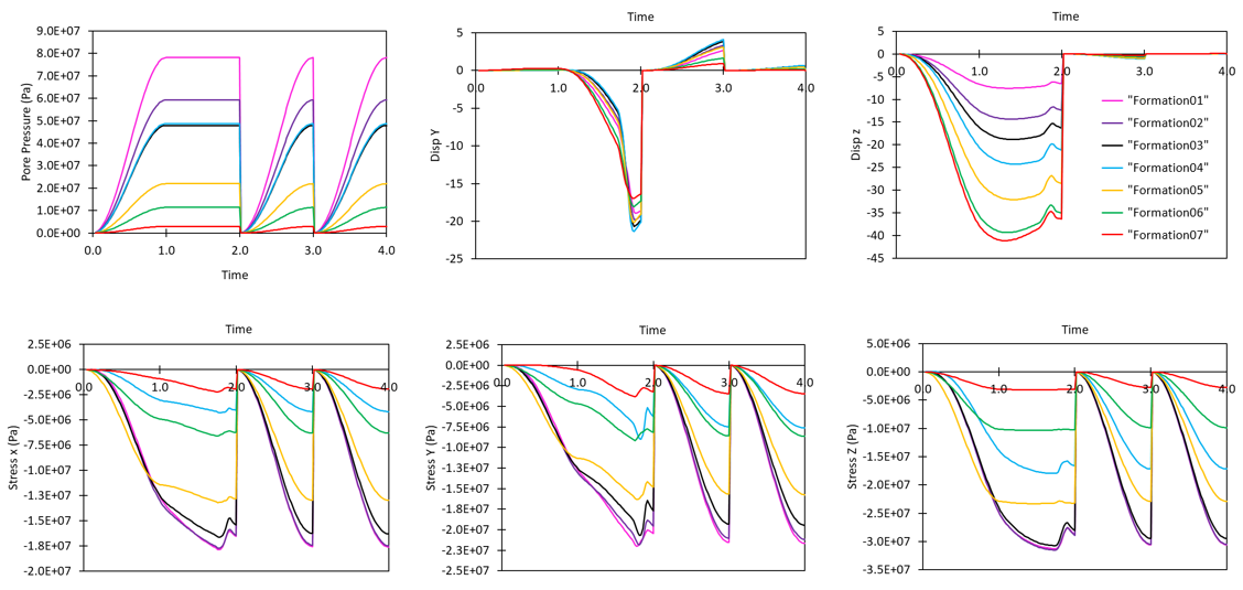
The results for the project are located in MEM_001\Case03\Results. In this directory the spreadsheet 00_MEM_001_Case03a_Results.xlsx contains all the processed history results output from the simulation. In the figure below some results for history points monitoring initialization are presented. The results show that the evolution of the different variables is in agreement with the conditions assumed for each stage, i.e.:
1.From t=0 to t=1 gravity is ramped up leading to stress increase. Pore pressure is also ramped up to initial value. The gravity stage leads to initial displacements which are dominant in the vertical (Z) direction as expected.
2.From t=1 to t=2 no stress change is imposed and pore pressure values are held over the duration of the stage. The contractional tectonic displacement is applied in the North-South direction (aligned with the Y axis) and this is reflected in the displacements and stress increase. Note the upward vertical displacement due to the Poisson ratio effects and layer thickening upon elastic tectonic deformation. Some "noise" is observed in the stress and displacement results at the end of the tectonic displacement stage but this amount of "noise" is not considered significant and has not impacted the stability of the stresses in later initialisation stages, else running more analysis steps in this stage will improved numerical stability.
3.From t=2 to t=3 contact is released from elastic to Coulomb properties. Stresses and pore pressure are ramped up from zero and displacements are reinitialized at the beginning of the stage. Note the development of positive displacements in the Y direction over the duration of the stage as the Coulomb fault behaviour lead to extensional fault slip as stresses increase (points are on the fault hanging wall which moves towards the positive Y direction).
4.From t=3 to t=4 stresses and pore pressure are ramped up from zero, displacements are reinitialized at the beginning and end of the stage and constitutive models are released from elastic to standard. Note that this has only implications for the reservoir which changes from elastic to poroelastic material, as the shale formations are all assigned elastic properties.

Evolution of properties during initialization stages.
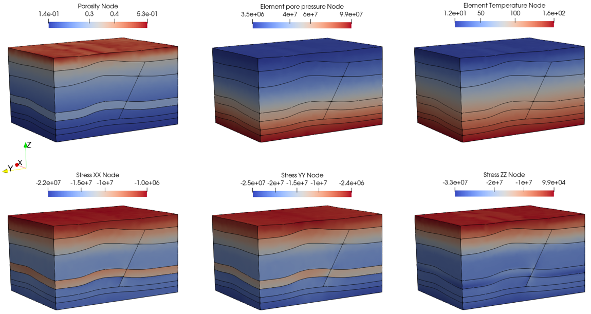
The figures below show the distribution of porosity, pore pressure, temperature and stresses after the initialization stages (simulation time 4). Note that the low horizontal stress values in the reservoir are due to the high overpressure.

Distribution of stresses, porosity, pore pressure and temperature at the end of initialization
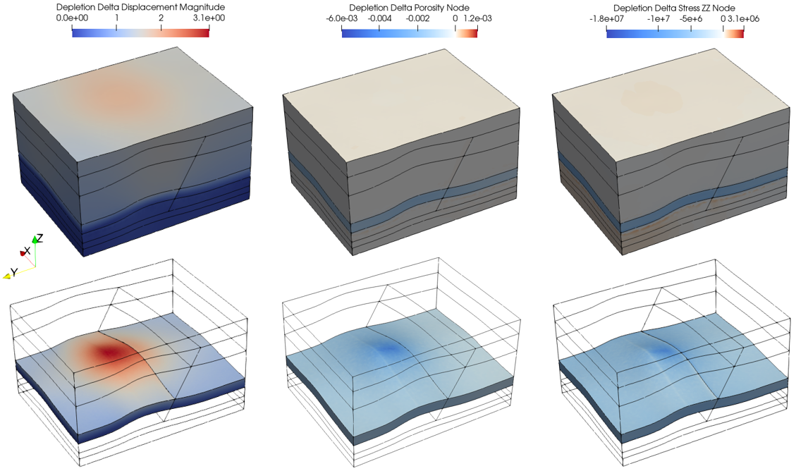
In the figures below, distribution of displacement change, porosity change and vertical stress change at the end of depletion are shown. Note that the change for horizontal stresses is not shown as it is not significant for the present case. Note also that these changes have been output because of the definition of the Reference_set_data. As expected, the drawdown at well 3 in the reservoir has led to a vertical effective stress increase in the reservoir which in turn has led to a porosity reduction due to elastic compaction (note the downward displacement).

Distribution of change in displacement, porosity and vertical stress at the end of depletion. The colour scale for plots showing the change in stress and porosity has been set so that the 0 value (no change) is shown in white, negative changes are shown in blue and positive changes in red.
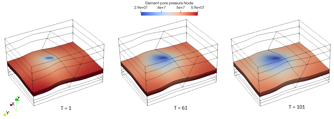
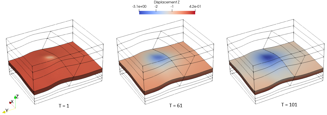
Following plots show the progression of pore pressure and vertical displacement over various depletion times (note the times "T" shown is simulation time minus initialization time 4). As expected, the maximum decrease in pore pressure is located around producer well 3 which was depleted by 20·106 Pa.


Progression of pore pressure and vertical displacement in the reservoir over depletion time.
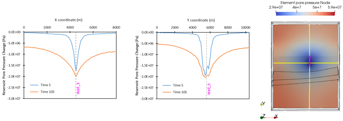
The change in pore pressure in the reservoir at the end of drawdown and depletion in the two history section line sets (yellow lines) are shown in the graph plots below. As can be seen in both profiles the maximum pore pressure change is concentrated at the producer well 3 location (indicated by the vertical discontinuous line) which is depleted by 20·106 Pa. This is also the location of maximum compaction and downward displacement as observed in the reservoir porosity change and displacement contour plots.

Pore pressure change in the reservoir monitored along the two history section line sets (shown in yellow) in the middle of the reservoir layer. The dotted line on the graphs indicate the coordinates where the two section lines cross at the well 3 location. Well 3 in the reservoir layer is shown in pink.

Porosity change and vertical displacements in the reservoir layer. History section line sets in the middle of the reservoir layer is shown in yellow and well 3 in the reservoir layer is shown in pink.
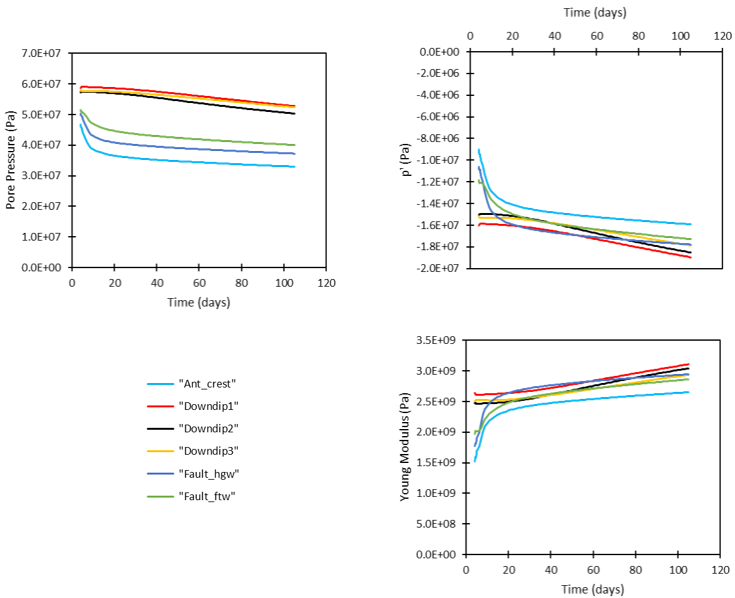
In the figures below, evolution of pore pressure, effective mean stress and Young's Modulus for the history points located within the reservoir is shown. As can be seen the reduction in pore pressure lead to an increase in effective mean stress which in turn lead to an increase in Young's Modulus due to the poroelastic law used to characterize the reservoir constitutive behaviour.

Pore pressure, effective mean stress and Young's Modulus history results at the six points located within the reservoir.
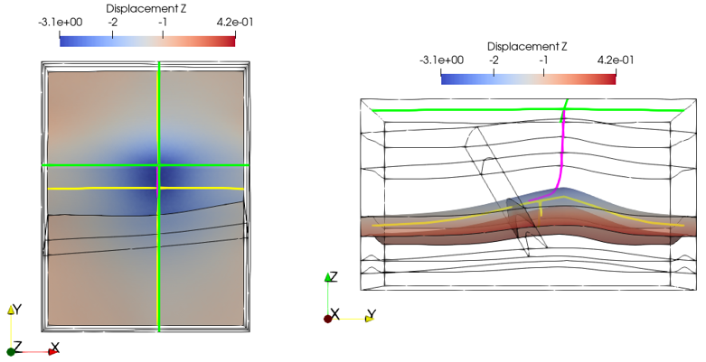
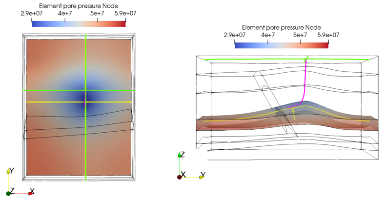
In the figures below, the maximum pore pressure change and vertical displacement is observed near well 3 located on the south-side of the anticline.


Pore pressure, displacement and location of well 3 (pink) in reservoir layer. History section lines for the reservoir is shown in yellow, crossing point at well 3 location. History section lines for the top surface is shown in green, this is vertically above the anticline crest.
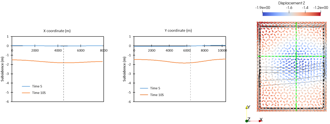
The subsidences at the end of drawdown and depletion in the two history section line sets on the top surface are shown below. As can be seen in both profiles, the subsidence increases with continued depletion of the reservoir (which lead to compaction and downward displacement). At the end of the simulation, the subsidence is marginally higher near producer well 3 where the maximum pore pressure change has occurred (as shown in the plots below and above).

Subsidence results monitored by the two history section line sets and vertical displacement at the top surface nodes. The dotted line indicate the coordinates where the two section lines cross (above the anticline crest). In the top surface plot the history section lines are shown in green.
The plots below show the progression of non-linear slip of the fault hanging wall at various depletion times. It can be observed that plastic slip (shown as contact net offset) occurs mainly in the reservoir layer and progressed initially from the producer well 3 location before spreading across the fault as the whole reservoir becomes depleted.

Progression of fault non-linear slip during depletion with friction coefficient of 0.2.
|
