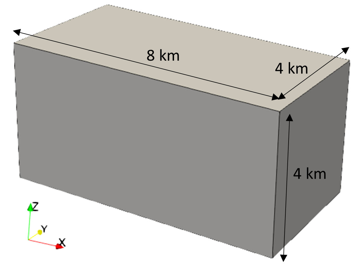
This tutorial example introduces the user to the usage of spatial grids to define properties in model domain space. Spatial grids are useful as they provide freedom to define properties in space which may not have a regular distribution (e.g. different property gradients with depth depending on location, lateral facies variations, etc). A simple geometry is defined consisting of a 3D rectangular prism of 8 km length, 4 km width and 4 km high. The geometry will be fully fixed and no loads will be considered thus focusing only on the spatial variation input. Spatial grids will be used to input distributions of porosity and volumetric plastic strain (for calculation of pre-consolidation pressure according to the hardening law).

 

Specific features considered in this example are:

1Definition and understanding of different types of spatial grids to input properties

2Definition of spatial plan to easily define lateral change in facies

3Use of spatial tables in order to define properties which may have up to 2 dependencies in other properties (e.g. permeability as a function of porosity, Young's modulus as a function of porosity and temperature, etc).

 

 

Geometry for tutorial example SpatVar_001

 

 

 

Simulation Cases

 

Case 1 Base Case description (Grid type 1)

 

Case 1b Base Case Grid defined at Cell centres

 

Case 2 Definition of Grid type 3 equivalent to Case1 grid (regular grid)

 

Case 3 Definition of non-regular Grid type 3

 

Case 4 Usage of Spatial table (property dependencies)

 

Case 5 Spatial plan to define lateral changes in properties

 

Case 6 Spatial grid group (grid defined by mesh topology at group basis)

 

Case 7 Mapping of values in non-conforming grids (domain larger than grid)