Case 1A Base Case Description

In ParaGeo the data concerning definition of the geometry is specified at the end of the data file, after the END DATA (which is a compulsory command indicating the end of the model general data and start of the model geometry data).

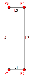
The geometry of the problem domain consists in a rectangular column defined by one surface, which is defined by four lines which connect four points and is identical to the geometry described in Mesh_001 (see that example for full description of the geometry data).

Points (nodes) and lines defining the model geometry

Mesh_control_data

The Mesh_control  data structure is compulsory and defines :

1The mesh generation algorithm type.  Valid values are:

•1 - Structured mesh generation

•2  - Unstructured mesh generation.

Structured_mesh_data

The structured mesh generation algorithm generates regular meshes on geometry defined using quadrilateral surfaces in 2-D or hexahedral volumes in 3-D.    The limitation of the algorithm is that the number of divisions on opposing lines in each surface must have the same number of divisions.  This is enforced by automatically evaluating sets of lines within the geometry that must have the same number of divisions.   This also simplifies the definition of the line division data, as only one line within any set needs to be assigned division data.  

In addition to defining the number of divisions on a line, a weighting for the distribution of the division size may also be defined using the Structured_line_set data structure.

The Structured_mesh_data  data structure defines:

1The default number of divisions for all geometry lines (Default_divisions).

2The list of sets of additional line division data sets (List_structured_line_sets) to be used to generate the mesh.

Structured_line_set

The Structured_line_set data structure defines:

1The  number of divisions for  geometry lines associated with this set (Number_divisions).

2The list of lines to which the structured line set will be applied.

ParaGeo groups are geometric regions with specific properties, material assignments, individual stratigraphy layers, etc. ParaGeo groups may encompass one or several surfaces in 2D problems and one or several volumes in 3D problems. Two compulsory data structures are used for the definition of ParaGeo groups; Group_data and Group_control_data

Group_data

The Group_data data structure is compulsory and defines the properties for each geometry group.  For this example these comprise:

1The name of the group.

2The element type.

3The material properties to be assigned to the group.

4The porous flow type which may be:

(a) 0 - Non-porous materials  - bulk density defined by the value specified in the grain density

(b) 1 - Dry porous material   - bulk density defined using grain density and porosity

(c) 2 - drained analysis with non-zero pore pressures (both grain density and fluid density must be specified)

(d) 3 - Undrained analysis (both grain density and fluid density must be specified)

(e) 4 - Coupled geomechanical/porous flow (both grain density and fluid density must be specified)

(f) 5 - Drained effective stress analysis (pore pressure not defined) - bouyant bulk density

5 The surface that defines the geometry for the group.

Group_control_data

The Group_control_data  data structure is compulsory and defines:

1The number of geometry groups in the problem, where each geometry group relates to a region with specific properties; e.g. regions with different material assignments, individual stratigraphy layers, etc.

2The group number.

3Whether the group is active or inactive in the fields; i.e. geomechanical, porous flow, thermal, that are being solved.

The Material_data data structure defines the properties of sandstone.  Only the data required for an elastic geomechanical analysis for a porous material is defined.  This comprises:

1The units of the material data

2Elastic properties

3Grain density (required for computation of the mass)

4Porosity

The Support_data data structure defines the entities which have some or all of their displacement freedoms prescribed.  While the Support_data identifies that specific freedoms are prescribed, if the prescribed value is non-zero then the magnitude of the prescribed value must be defined using the Global_loads data structure.

Standard load types are defined using three data structures:

1Global_loads which defines the load and the assignment to geometry entities,

2Time_curve_data which defines the variation of the load magnitude with time,

3Load_case_control_data which defines which load cases are active in the analysis step

Global_loads

Global_loads data structure may be used to define a wide range of loading boundary conditions (i.e. Stress load, displacement load, pore pressure load, temperature load, etc). In this case it is used to define a stress load applied to the top surface line.

Time_curve_data

The Time_curve_data defines the rate and magnitude of the load applied. Each load case must have an associated time curve with the same ID number; i.e. load case Global_loads NUM=1 is always assigned Time_curve_data NUM=1.

Load_case_control_data

High definition history data is used to both:

1Construct graphs of key variables for result interpretation.

2Monitor the dynamics in the solution for quasi-static analysis.

Two methods are usually adopted for monitoring dynamic response in  quasi-static analysis using a dynamic solver:

1Visualization of time histories of the kinetic and elastic strain energy.  These provide a global measure of the dynamic response for the complete problem domain.

2Visualization of point values of displacement, velocity or stress at specific points within the problem domain.  These provide  a local measure of dynamic response and can identify  small regions of active deformation which exhibit a dynamic response within a largely quasi-static domain.   This localized dynamic response may be difficult to discern using the global measures when the majority of the domain is behaving quasi-statically.

History_point

The History_point data structure allows creation of time history sets of specific results for individual points.  The points are defined by a point label and coordinates and are automatically located within the element discretisation.  The time history data is written as an ASCII file in comma delimited column format to: datafile_number.hdh where datafile is the data file name and number is the History_point set number.

Several History_point data structures may be specified and additional sets may be added during the analysis.

History_global

The History_global data structure creates a time history set with quantities that is applicable to the complete domain; e.g. total kinetic energy. The time history data is written as an ASCII file in comma delimited column format to: datafile_000.hdh where  datafile is the data file name.

The Control_data data structure defines the solution algorithm and output requirements for the geomechanical field.  Several Control_data structures can be defined, with each data structure defining a stage or "step" in the analysis; e.g. stage 1 may be an initialization step and stage 2 may be a loading step. Once a Control_data keyword, or a group of control keywords in a coupled problem, is processed, ParaGeo processes this control step before reading any further data from the data file.  For the geomechanical field the key parameters are:

1The solution algorithm (Solution_algorithm) - Several different algorithms may be used with the simplest being type 1 - Standard Explicit Dynamic Solver.  This solution algorithm is conditionally stable with stability governed by a critical time step (Δtcrit).

2The factor of critical time step (Factor_critical_time_step) - The critical time step can only be evaluated approximately.  Consequently the time step is evaluated as Δt = fcritΔtcrit where fcrit is  the factor of critical time step  where fcrit < 1.0. The default value is 0.9 in 2-D and 0.7 in 3-D. Lower values are sometimes required if the response is highly nonlinear.

3Termination data for the stage (via Maximum_number_time_steps and Termination_time) - Generally the stage is terminated based on time and the maximum number of time steps is only required in nonlinear problems undergoing large deformations; i.e. when there is potential for the time step to become very small leading to an excessively large number of time steps.

4Plot file output (via Output_frequency_plotfile  and Output_time_plotfile) - note that setting the output frequency for the plot file to -1 enforces output on the last analysis step.

5Screen message output (Screen_message_frequency) - sets the number of steps before a status summary is written to the Command window.

The END DATA command signifies the end of the analysis data file and the start of the geometry definition.