Case01 Base Case

Contents

The data file for the project is: Intro_001\Case01\Data\Intro_001_Case01.dat.

Basic Set Up: Data File Description

The description of the datafile is provided here in an order that facilitates understanding of the model definition (e.g. geometry first, then mesh, then groups, etc.) but the actual data may be placed in a different order within the datafile.

Geometry definition data

In ParaGeo the data concerning definition of the geometry is specified at the end of the data file, after the END DATA (which is a compulsory command indicating the end of the general data for the model and the start of the model's geometry data).

The geometry of the problem domain is defined in terms of simple geometrical entities; i.e. points (vertices), lines, surfaces and volumes arranged in a hierarchical manner; i.e. points are used to define lines, lines are used to define surfaces and surfaces are used to define volumes. The geometry entities comprise:

1Points (Geometry_vertex or Nodal_data).

2Lines (Geometry_line) - either linear, parametric or polylines defined using the points.

3Surfaces (Geometry_surface)- bounded by lines and defined as either parametric or tesselated.

4Volumes (Geometry_volume) - closed volumes defined by surfaces.

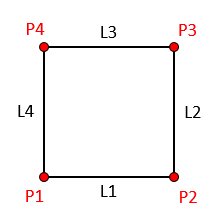
For the current problem a single rectangular surface is required which is defined by four lines. Consequently four points must also be defined (see the figure below).

Intro_002

Points (nodes) and lines defining the model geometry

Nodal_data

The Nodal_data data structure defines the coordinates of the points defining the geometry.

Data File

* Nodal_data

node_numbers IDM=4

1 2 3 4

coordinates IDM=3 JDM=4

0.0 0.0 0.0

1.0 0.0 0.0

1.0 1.0 0.0

0.0 1.0 0.0

1.In Node_numbers keyword the node numbers for the four nodes are defined

2.The four points coordinates are defined as shown in the following table:

Point	X-Coordinate	Y-Coordinate	Z-Coordinate
1	0.0	0.0	0.0
2	1.0	0.0	0.0
3	1.0	1.0	0.0
4	0.0	1.0	0.0

Geometry_line

The Geometry_line data defines the topology of the four lines consisting in the base, top and sides of the model surface.

Data File

* geometry_line NUM=1

line_type 1

points IDM=2

1 2

* geometry_line NUM=2

line_type 1

points IDM=2

2 3

* geometry_line NUM=3

line_type 1

points IDM=2

3 4

* geometry_line NUM=4

line_type 1

points IDM=2

4 1

1.Each of the four lines defining model boundaries are defined which are assigned ID numbers 1, 2, 3 and 4.

2.Each line is connecting two points.

3.Line_type 1 keyword defines that the line is a linear line connecting two points.

Geometry_surface

Data File

* geometry_surface NUM=1

lines IDM=4

1 2 3 4

1.The model domain is defined by a single rectangular surface which is assigned ID number 1 (NUM=1)

2.The surface is defined by lines 1, 2, 3 and 4.

Mesh definition data

The current example considers a single 4-node element (structured mesh). Two data structures are required to define mesh generation: Mesh_control_data and Structured_mesh_data

Mesh_control_data

The Mesh_control_data data structure is compulsory and is used to define the mesh generation algorithm type. Valid values are:

•1 - Structured mesh generation

•2 - Unstructured mesh generation.

Data File

* Mesh_control_data

! ---------------------------------

Generation_algorithm 1

1.For the present case a structured mesh generation algorithm is used

Unstructured_mesh_data

The Structured_mesh_data data structure is used to define the default number of divisions. Note that generally the number of divisions for the different lines may be different and in such case additional should be specified.

* Structured_mesh_data

! ---------------------------------

Default_divisions 1

1.In the present case only one division is used (single element)

Data for definition of Groups

ParaGeo groups are geometric regions with specific properties, material assignments, individual stratigraphy layers, etc. ParaGeo groups may encompass one or several surfaces in 2D problems and one or several volumes in 3D problems. Two compulsory data structures are used for the definition of ParaGeo groups; Group_data and Group_control_data

Group_data

The Group_data data structure is compulsory and defines the properties for each geometry group. For this example these comprise:

1The name of the group.

2The element type.

3The assigned material.

4The surface that defines the geometry for the group.

5The porous flow type

* Group_data NUM=1

! ---------------------------------

Group_name "sand"

Element_type "QPM4"

Material_name "Elastic"

Surfaces IDM=1

Porous_flow_type 1

1.Group 1 (NUM=1) is named "sand" and is defined using the QPM4 element (4 node Plane Strain element).

2.The assigned material is named "Elastic"

3.The geometry of the group is defined by surface 1.

4.The porous flow type is set to 1 (dry porous material)

Group_control_data

The Group_control_data data structure is compulsory and defines:

1The number of geometry groups in the problem, where each geometry group relates to a region with specific properties; e.g. regions with different material assignments, individual stratigraphy layers, etc.

2The group number.

3Whether the group is active or inactive in the fields; i.e. geomechanical, porous flow, thermal, that are being solved.

Data File

* Group_control_data

! ---------------------------------

Group_numbers IDM=1

Active_geomechanical_groups IDM=1

The problem has a single group (Group 1) that is active in the geomechanical field.

Material_data

The Material_data is used to define the material properties. Note that several Material_data data structures may be defined in a given datafile but only those assigned to ParaGeo groups will be used.

Data File

* Material_data NUM=1

! -----------------------------------

Material_name "Elastic"

! --------------------------------------------------------

Grain_stiffness 20000 ! MPa

Grain_density 2650.0 ! Kg/m3

! --------------------------------------------------------

Porosity_model_type 1 ! Constant Porosity

Porosity 0.40

! --------------------------------------------------------

Elastic_model_type 1 ! Isotropic Elasticity

Elastic_properties IDM=2

/Young's Modulus (E)/ 1000.0 ! MPa

/Poisson's Ratio (V)/ 0.25

1.The material is named "Elastic"

2.Grain properties are defined; a grain stiffness of 20000 MPa and a grain density of 2650 Kg/m3

3.The porosity specified is 0.40.

4.Isotropic elasticity model is defined with a Young's modulus of 1000 MPa and a Poisson's ratio of 0.25

Data defining boundary conditions

Support_data

The Support_data is used to:

1.Define sets of displacement constraints

2.Assign a set of displacement constraints to model lines.

Data File

* Support_data

! ---------------------------------

Displacement_codes IDM=3 JDM=4

/Set 1/ 1 0 0

/Set 2/ 0 1 0

/Set 3/ 1 1 0

/Set 4/ 0 0 0

Displacement_code_lines IDM=4 JDM=2

/lines/ 1 2 3 4

/Assign Set/ 2 1 2 1

1.Four different displacement constraint sets are defined. Each set defines whether displacement in X, Y and Z directions is constrained (1) or not (0).

2.Lines 1 and 3 (base and top respectively) are assigned displacement code number 2 which constrains displacement in Y direction.

3.Lines 2 and 4 (side boundaries) are assigned displacement code set number 1 which constrains displacement in X direction.

Loading data

The loading data defined comprises:

1.A Global_loads data structure

2.The corresponding Time_curve_data defining the loading rate

3.The Load_case_control_data data structure defining whether the defined Global_loads in the datafile will be active (2) or not (0).

Data File

* Global_loads NUM=1

! ---------------------------------

Prescribed_displacement IDM=2 JDM=1

/Set 1/ 0.0 -0.05

Pres_displacement_lines IDM=1 JDM=2

/lines/ 3

/Assign Set/ 1

* Time_curve_data NUM=1

! --------------------------------------

Name "Loading"

Curve_type 1 ! PiecewiseLinear

Time_curve IDM=3

0.0 1.0 2.0

Time_factor IDM=3

0.0 1.0 1.0

* Load_case_control_data

! ---------------------------------

Loadcases IDM=1

Active_load_flags IDM=1

1.A Global_loads data structure to prescribe displacements is defined.

2.A set with a prescribed vertical downward displacement of 0.05 m is defined.

3.The displacement set is assigned to line 3 (which is the top).

4.Time_curve_data NUM=1 to define loading rate for Global_loads NUM=1 is defined.

5.Curve_type 1 is set (piece wise linear curve)

6.The displacement will be ramped up from time 0 to time 1 and then will be held constant from time 1 to time 2.

7.In Load_case_control_data we define that Global_loads NUM=1 (Loadcases 1) is active (load flag 2).

History output data

A History_point data structure is defined. This data is used to output the evolution of the specified variables at a specified point location. Note that the point is not fixed in the space and it moves with deformation.

Data File

* History_point NUM=1

! ---------------------------------

Name "Set1"

Group 1

Output_frequency_time 0.01

Point_coordinates IDM=2 JDM=1

1.0 1.0

Displacements IDM=1

"Disp_y"

Stresses IDM=3

"Strs_xx" "Strs_yy" "Strs_zz"

Strains IDM=2

"Strn_xx" "Strn_yy"

Stress_invariants IDM=2

"Press" "Efstrs"

Element_data IDM=1

"Porosity"

1.A history point with NUM=1 is defined. This will output results to a file named "Intro_001_Case01_001.hdh" (a history point with NUM=2 would output the results at a file named "Intro_001_Case01_002.hdh"). In general History_point data outputs the results to a file named DataFileName_NUM.hdh.

2.The name of the history point set is "Set1".

3.The history point set is assigned to group 1.

4.Results will be output every 0.01 time units.

5.A single point with coordinates X=1.0 Y=1.0 is defined (top right corner of the model).

6.Several variables are output (see the History_point page from the reference manual for the list of variables and keywords).

Control_data

At least one solution control data structure must always be specified. This data structure defines the end of each simulation stage. For each stage this data structure defines the solution algorithm, termination time, step control and output frequency data for screen, plot file and restart fields.

As mentioned at the initial guidelines, once a control data keyword is processed, ParaGeo processes this control step (simulation stage) before reading any further data from the data file.

Data File

* Control_data

! ===================================

Control_title "Stage 1"

Solution_algorithm 1

Factor_critical_time_step 0.7

Maximum_number_time_steps 1E8

Target_number_time_steps 20000

Duration 1.0

Output_time_plotfile 0.2

Output_frequency_plotfile -1

Screen_message_frequency 1000

1.Control data for the geomechanical field is specified for two stages.

2.Solution_algorithm is set to 1 (transient dynamic algorithm).

3.Factor_critical_time_step and Maximum_number_time_steps will be discused in Mech_001 tutorial example.

4.Each stage is set with a duration of 1.0 time units.

5.Target_number_time_steps defines the number of mechanical time steps to be used to solve the current simulation stage.

6.Output_time_plotfile is set to 0.2 so a plot file will be output every 0.2 time units.

7.Output_frequency_plotfile indicates the number of time steps between consecutive output of plot files. If set to -1 a plot file will be output at the end of the stage.

8.Screen_message_frequency defines the number of time steps between every print of simulation information to the screen (command prompt).

END DATA

The END DATA command signifies the end of the analysis data file and the start of the geometry definition.

Data File
END DATA	The END DATA command is compulsory

Results

The results for the simulation are in Intro_001\Case01\Results. There are several result files output from the simulation:

•Intro_001_Case01_No.plt : Binary plot file where No is the plot file number. Plot files contain the element and nodal results for all output variables.

•Intro_001_Case01_No.xmf : Plot file description for plot file number No. This file can be loaded in ParaView to visualise plot file number No.

•Intro_001_Case01_No.gmr : Binary geometry plot file where No is the geometry plot file number. Geometry plot files contain the geometry results (i.e. line numbers, line length, surface numbers, etc).

•Intro_001_Case01_gmr_No.xmf : Geometry plot file description for geometry plot file number No. This file can be loaded in ParaView to visualise geometry plot file number No.

•Intro_001_Case01_001.hdh : History result file for history point NUM=1. This file contains results in a comma separated value format and can be opened with Excel.

•Intro_001_Case01.res : Simulation log file. This file contains information on data reading and processing, time steps, etc. If an error occurs during the simulation (shown by a Fatal Error message in the command prompt) an error message will be written which may provide a clue on what is causing the error.

We open the history results file (Intro_001_Case01_001.hdh) in excel and plot the evolution of some variables with time as shown in the figure below. Note that the history monitoring point is located in the top right corner of the model domain.

Intro_004

Evolution of displacement, porosity and stress results with time.

As can be seen the point has experienced a downward (negative) vertical displacement of 0.05 m that is applied from t=0.0 to t=1.0 and then kept constant until end of simulation at t=2.0. This is consistent with what was specified in the Global_loads and Time_curve_data.

Porosity and stress results are also plotted. As can be seen the prescribed displacement has lead to a compressive stress increase in both X and Y directions (negative sign indicates compression whereas a positive sign indicates tension). Horizontal stress has increased due to the Poisson ratio effect when compressing in the vertical direction and constraining horizontal extension with the roller boundary condition. The elastic compaction has led to a Porosity decrease.

You may open the file Intro_001_Case01.xmf in ParaView (by either dragging the file within a ParaView window or by going to File/Open... and then select the file in ParaView). Note that when prompted the XDMF Reader option must be selected. At the top center of the ParaView window, below the menus bar there should be the following icons:

ParaView VCR and Current time controls

Those icons and menus allow to navigate through the different plot files and select the time to be visualised. If we click on the icon the last plot file will be displayed. This plot file corresponds to Time 2 (also selectable from the corresponding drop down menu) and the plot file number 10 (number 9 in ParaView as in ParaView plot files are numbered starting from 0 as opposed to ParaGeo plot file numbers which start from 1).

In the row of icons below, you can find the active variable and representation drop down menu as shown in the image below. You can select nodal variable displacement and then you should be able to select Y direction instead of Magnitude. It should be noted that variables preceded by are nodal averaged variables whereas variables preceded by are element variables.

ParaView active variable and representation drop down menus

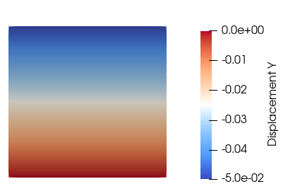
Below there is a figure showing the vertical displacement at the last output time. As can be seen the downward displacement is maximum at the top surface and decreases linearly to 0 towards the base.

Intro_005

Vertical displacement at time t=2.0