Geol_002 Geological Modelling with Zmap Import
Note: The present tutorial example is only recommended to advanced users already familiar with ParaGeo.
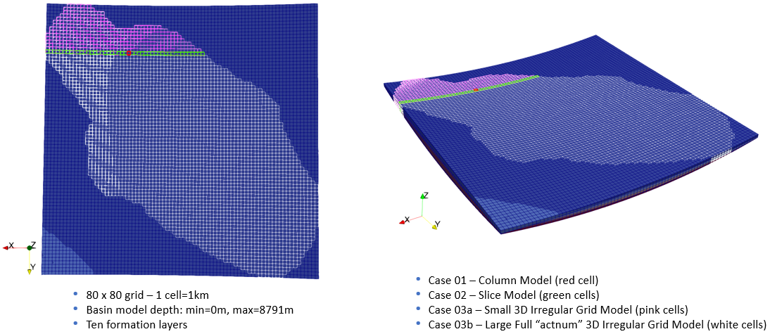
In the present tutorial example a geological basin modelling workflow incorporating Zmap file import in ParaGeo will be demonstrated. Four case models are presented in this tutorial example (see figure below):
1Case01 - 3D column model with 5x5 grid mesh (red cell).
2Case02 - Pseudo-3D slice model (green cells).
3Case03a - Small 3D irregular grid model with 'ragged' boundaries (pink cells).
4Case03b - Large 3D irregular grid model with 'ragged' boundaries (white cells).

Full Basin Model showing Four Extracted Sub-model Cases
Features of the example are:
1Utility to import Zmap files and output to ParaView plot file and Abaqus file incorporating various functionalities, e.g. sub-grid extraction, grid subdivisions, actnum functionality, horizontal horizon extraction for column, etc.
2Restoration modelling (geomechanical only).
3THM sedimentation modelling.
4Kerogen oil and gas generative layer for hydrocarbon generation.
5Basal thermal flux.
6Hexahedral mesh model.
7Moving water table with time.
8Directional decompaction.
9Multi-material layer model with permeable (sandstone), impermeable (shale) and facies mixture layers.
10Boundary node extraction functionality for irregular grid hex models with 'ragged' boundaries.
Geomechanical restoration and THM-coupled forward simulation is to be performed on sub-models derived from a pseudo ten formation layer geological basin model 80 x 80 grid cells (1 cell=1km) with model depths 0 - 8.791km. These models are extracted using ParaGeo utilities for importing zmap horizons in conjunction with Eclipse data import. In the creation of these models, various utility functionalities are demonstrated - these include: sub-grid extraction, grid subdivisions, actnum (active flag) functionality, horizontal horizon extraction for column model, etc. Four 3D case models are investigated in rising complexity and size, from column to slice model to small and finally large irregular grid 3D models with 'ragged' side boundaries. The large model has 421,025 elements. In order to be able to simulate large geological basin models with reasonable number of elements, hexahedral mesh is utilised in all models as it is requires the least elements.
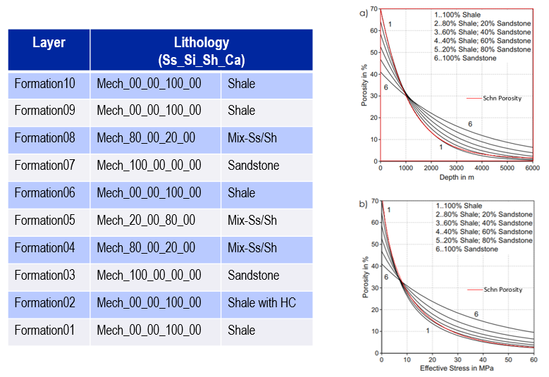
The models in this example incorporate a moving water table with water level rising from 1000m to 2000m above a reference point over a specified time period, and a basal thermal flux loading of 0.056W/m2. Directional strain decompaction of 3% is included in all models with the exception of the column model as it does not add anything and is generally not performed for a column model. The basin has ten multi-material formation layers represented with different facies mixtures - two permeable/flow sandstone layers sandwiched in between impermeable/barrier shale layers and inclusion of a kerogen 'B' oil and gas generative layer for hydrocarbon generation (see picture below).
Support conditions for the models differ: •In the column model, horizontal fixities normal to the plane are defined for all four side boundaries during restoration and the top of the sediments are coupled in Z during deposition. •In the slice model, the "North" and "South" boundaries are fixed in Y, the "East" boundary is fixed in X and the "West" boundary is prescribed coupled freedom in X during restoration. •In the 3D irregular grid model, two sides are fixed during restoration - the "South" boundary is fixed in Y and the "East" boundary is fixed in X. During forward simulation, the side boundary nodes for the 'ragged' boundaries will be extracted using a special utility to apply the restoration displacements.
Notional well lines are represented with history section lines along the length of the model and monitored for various defined variables, e.g. temperature, pore pressure, porosity, stresses and kinetic KTR. These are output in .las format at the end of every stage. A point in every formation layer is also monitored for evolution of temperature, pore pressure, porosity, stresses and strains. Reference set data to output the change in selected variables is also defined.
Units of the model for stress, length, time and temperature are MPa, m, Ma and Celsius respectively.
Layer Lithologies and Material Properties The four lithologies for the ten formation layers are represented as percentages of Sandstone-Siltstone-Shale-Carbonate (Ss_Si_Sh_Ca) mixtures (see table below). The porosity depth and effective stress trends for various facies mixtures are also shown in the plots below.
Formation Layer Lithologies and Porosity Depth and Effective Stress Trends for Various Facies Mixtures
All materials utilize a poro-elastoplastic constitutive SR4 plastic material model with hardening data based on the Cam Clay analytical model. The material property parameters for the defined materials are (NB: where not shown, similar values to the first column material are defined):
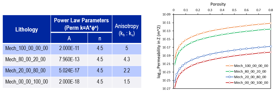
A transverse isotropic porosity dependent permeability relationship based on the Power Law is also utilized for the materials defined as shown in the figure below. The horizontal to vertical permeability ratios are also indicated.
Transverse Isotropic Porosity Dependent Material Permeabilities based on Power Law
The additional material parameters related to the porous flow and thermal fields are (NB: where not shown, similar values to the first column material are defined):
Fluid Properties The properties of the pore fluid must be specified. The principal parameters are:
|
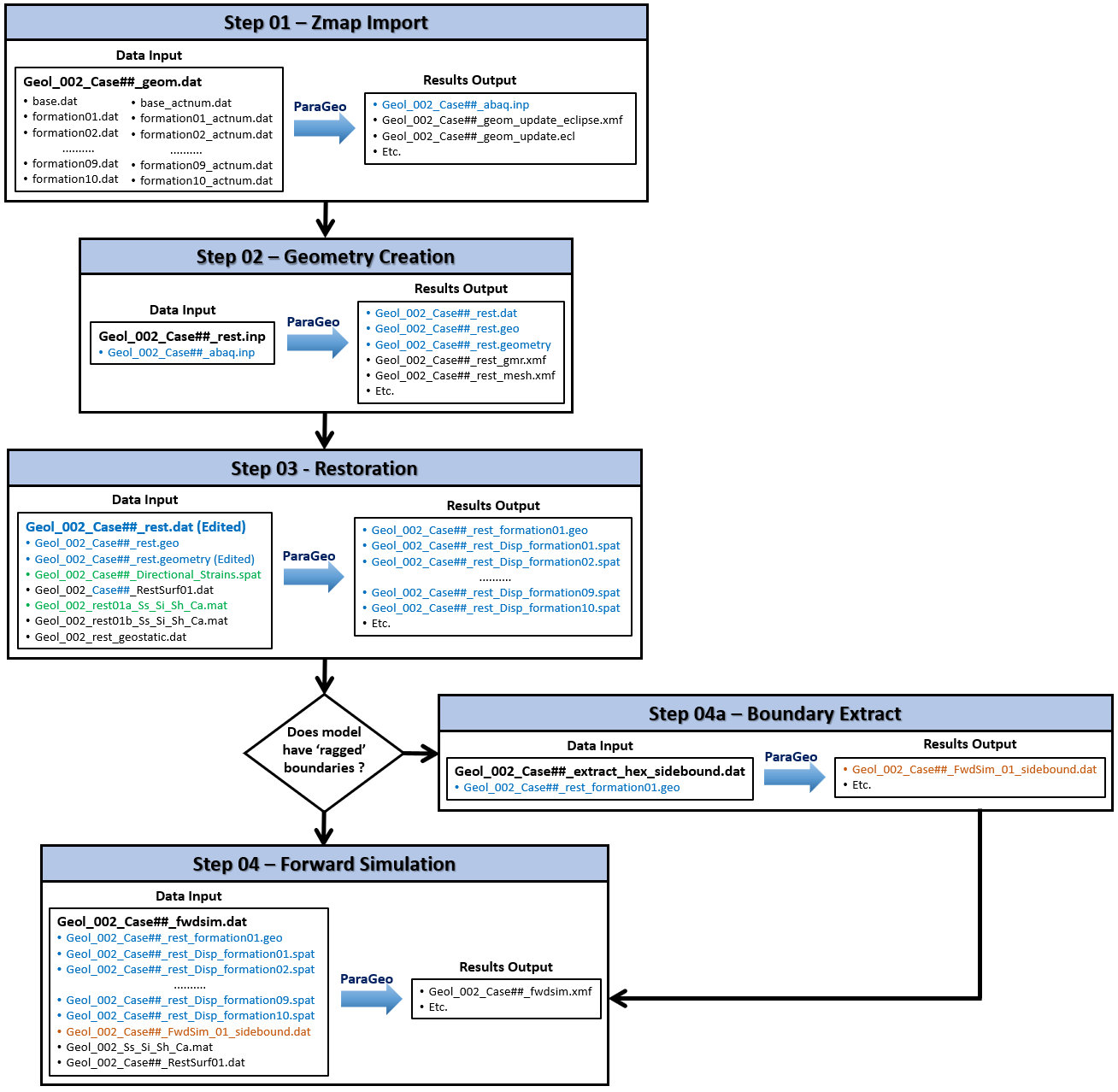
The workflow for all case examples encompass the following four main steps which is summarised in the flowchart below. The text in blue in results are output files which are utilised in data input in the next step. Text in green in data input are required for directional strain decompaction in geomechanical restoration and text in brown in results are output files containing side boundary nodes which are utilised in the forward simulation data input for 'ragged' boundary models. 1Step 01 - Zmap file import and output to Abaqus input .inp file. 2Step 02 - Conversion of .inp file to suitable ParaGeo geometry (.geo and .geometry) files and data .dat file. 3Step 03 - Geomechanical restoration of the defined 3D geological structure. 4Step 04 - Forward simulation of the sedimentation process (THM modelling). Step 04a - Extraction of side boundary nodes for 'ragged' boundary models. Note that this is valid for hex mesh only and performed for models with 'ragged' boundaries. It is to be carried out prior to performing Step 04.
Workflow Flowchart for Geological Basin Modelling with Zmap Import
|
Simulation Cases
The simulation files for the four case models are found in: ParaGeo_Tutorial_Examples\Geol_002.
A full description of the data required for the column model is provided in Case01 Column Model description. Subsequent cases will only contain description of additional data or data different to the preceding case model in increasing complexity. To this end, the user is recommended to work through each of the case examples relevant to the required target model.
The following table shows the run statistics for the four simulation cases on a single processor :

Run statistics for simulation cases on single 3.6 GHz AMD processor
Notes on parallel simulation:
Solver |
Advantage |
Disadvantage |
Mumps (Default) |
•More likely to give answers if problem is poorly conditioned |
•Takes much more memory for large problems •Likely to fail in parallel for large problems (Windows only) |
Petsc
* Solver_control NUM=1 ! -------------------------------------- Solver_type "Petsc" |
•Generally quicker if solution can converge •Uses less memory for large problems |
•May not converge for poorly conditioned problems |
Case 03a 3D Small Irregular Grid Model with 'Ragged' Boundaries
Case 03b 3D Large Irregular Grid Model with 'Ragged' Boundaries


