Case02 Usage of geometry sets

Contents

The data file for the project is: Intro_001\Case02\Data\Intro_001_Case02.dat. It is assumed that the user has undertaken Case01 first. Most of the data in the data file is identical to such case and hence full description of the datafile is not provided here. In the present case the focus is made on:

1.Definition of several ParaGeo groups

2.Definition of geometry sets and its usage for application of boundary conditions

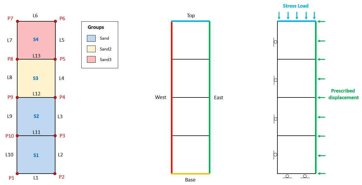
The model geometry is defined as shown in the figure below. The domain is defined via 4 surfaces (S1, S2, S3 and S4). Those surfaces will be used to define 3 ParaGeo groups (Sand, Sand2 and Sand3) each one defined by a single element. Geometry sets will be defined for all model boundaries and will later be used to facilitate definition of the boundary conditions. Boundary conditions will consist of rollers at the base and West boundary, a stress load that will be applied from time t=0.0 to t=1.0 and then held constant until t=2.0 and a displacement boundary condition applied on the East boundary from t=1.1 to t=2.0.

Intro_011

Model geometry and groups (left), geometry sets (middle) and boundary conditions (right)

Definition of multiple ParaGeo groups

The present case considers 3 ParaGeo groups. The set up of the Group_data and Group_control_data is shown below.

Group_data

Data File

* Group_data NUM=1

! ---------------------------------

Group_name "Sand"

Element_type "QPM4"

Material_name "Elastic"

Surfaces IDM=2

1 2

Porous_flow_type 1

* Group_data NUM=2

! ---------------------------------

Group_name "Sand2"

Element_type "QPM4"

Material_name "Elastic2"

Surfaces IDM=1

Porous_flow_type 1

* Group_data NUM=3

! ---------------------------------

Group_name "Sand3"

Element_type "QPM4"

Material_name "Elastic"

Surfaces IDM=3

Porous_flow_type 1

•Three Group_data data structures are defined with names Sand, Sand2 and Sand3 and assigned ID numbers 1, 2 and 3 respectively.

•Group "Sand" is defined by surfaces 1 and 2, group "Sand2" is defined by surface 3 and group "Sand3" is defined by surface 4.

•Groups "Sand" and "Sand3" are assigned "Elastic" material whereas group "Sand2" is assigned "Elastic2" material. Both materials have same properties except Young's modulus which is 1000 MPa for "Elastic" and 2000 MPa for "Elastic2".

Group_control_data

Data File

* Group_control_data

! ---------------------------------

Group_numbers IDM=3

1 2 3

Active_geomechanical_groups IDM=3

1 1 1

•The three groups previously defined are defined as active for the geomechanical field.

Definition of geometry sets

Geometry sets allow to define sets of geometry entities that later can be used to define boundary conditions, assign properties, etc. Geometry sets may contain several points, lines, surfaces and volumes (including combinations of those). Below the definition of geometry sets for the four model boundaries are shown.

Data File

* Geometry_set NUM=1

! ---------------------------------

Name "Base"

Lines IDM=1

* Geometry_set NUM=2

! ---------------------------------

Name "Top"

Lines IDM=1

* Geometry_set NUM=3

! ---------------------------------

Name "East"

Lines IDM=4

2 3 4 5

* Geometry_set NUM=4

! ---------------------------------

Name "West"

Lines IDM=4

7 8 9 10

•Geometry sets for the four model boundaries are defined.

It should be noted that a given geometry entity may be included in more than one geometry set (e.g. lines 2 and 3 may be included also in an additional geometry set that we will call "East_bottom" in addition to the already defined "East").

Usage of geometry sets in defining boundary conditions

The defined geometry sets may be used to assign boundary conditions for example. This is illustrated here:

Support_data

Data File

* Support_data

! ----------------------------------------

Displacement_codes IDM=3 JDM=4

/Set1/ 1 0 0

/Set2/ 0 1 0

/Set3/ 0 0 1

/Set4/ 1 1 0

Displacement_code_geom_set IDM=3

"Base"

"East"

"West"

Displacement_code_geom_ass IDM=3

2 1 1

•Four displacement code sets are defined.

•Displacement code set 2 (displacement constrained in Y direction) is assigned to "Base" geometry set.

•Displacement code set 1 (displacement constrained in X direction) is assigned to geometry sets "East" and "West".

•"Top" is not assigned any displacement constraint.

Loading data

Data File 1

* Global_loads NUM=1

! ---------------------------------

Surface_load IDM=2 JDM=1

/Set 1/ 1.0 0.0

Surface_load_geom_set IDM=1

"Top"

Surface_load_geom_ass IDM=1

* Time_curve_data NUM=1

! --------------------------------------

Name "Stress load"

Curve_type 2 ! S-curve

Time_curve IDM=2

0.0 1.0

Time_factor IDM=2

0.0 30.0

* Global_loads NUM=2

! ---------------------------------

Prescribed_displacement IDM=2 JDM=1

/Set 1/ 1.0 0.0

Pres_displacement_geom_set IDM=1

"East"

Pres_displacement_geom_ass IDM=1

* Time_curve_data NUM=2

! --------------------------------------

Name "Displacement"

Curve_type 2 ! S-curve

Time_curve IDM=2

1.1 2.0

Time_factor IDM=2

0.0 -0.05

* Load_case_control_data

! ---------------------------------

Loadcases IDM=2

1 2

Active_load_flags IDM=2

2 2

•Global_loads with ID number 1 defines the stress load at the top surface (geometry set "Top").

•In Surface_load keyword the two numbers correspond to the stress normal and tangential to the surface respectively. The normal stress is set to 1.0 as the actual stress magnitude will be defined in Time_factor keyword within Time_curve_data.

•In Time_curve_data NUM=1 a magnitude of 30 MPa applied from t=0.0 to t=1.0 for the top surface stress is defined. It should be noted that stress loads are defined in a local coordinate system so that a positive number indicates a direction within the surface.

•Curve_type is set to 2. This defines an S-curve shape between 2 points.

•It should be noted that Time_curve_data works in such a way that the time factor 30.0 will be kept constant beyond last time defined corresponding to t=1.0.

•Global_loads number 2 defines the horizontal compressive displacement applied on the "East" boundary.

•A single prescribed displacement set is defined. The displacement in X direction is set to 1.0 as the actual magnitude will be defined in the Time_factor within the corresponding Time_curve_data.

•A displacement of 0.05 m towards the left (negative sign) is applied from t=1.1 to t=2.0 following an S-curve function (Curve_type set to 2).

•In Load_case_control_data, Global_loads with ID numbers 1 and 2 are defined active for the simulation.

•It can be noted that even though the Global_loads 2 takes place during the second simulation stage (which corresponds to t=1.0 to t=2.0) it may be defined before the first Control_data data structure.

Results

The results for the simulation are in Intro_001\Case02\Results.

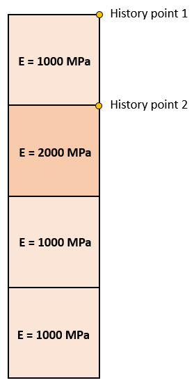
In the file Intro_001_Case02_001.hdh there are the results for the History_point set data number 1 which in this case is set to output results at two point locations. Point 1 is located at the top right corner of group 3 (surface number 4) whereas Point 2 is located at the top right corner of group 2 (surface number 3). Note that point 2 is located in the group that has assigned material properties named "Elastic2" which has a Young modulus of 2000 MPa instead of 1000 MPa (see the picture below). Also note that in the file the columns show the results following an order such as: Disp_x (point 1), Disp_x (point 2), Disp_y (point 1), Disp_y (point 2), etc.

Intro_012

Young modulus of each element and location of the two history points

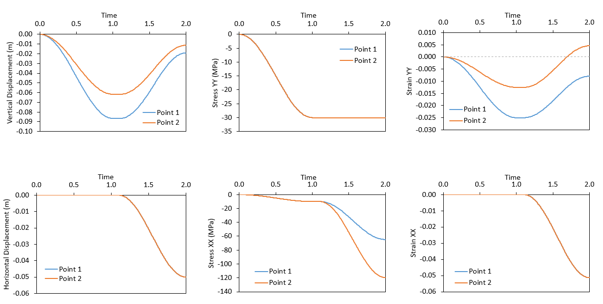
Below the history results for vertical and horizontal displacements, stresses and strains are plotted for the two points. It can be seen that:

1.Stress YY evolution for the two points is consistent with the load prescribed by Global_loads and Time_curve_data number 1 in which a stress of 30 MPa is applied at the top surface and is ramped up from t=0 to t=1 following an S-shape curve and then kept constant. The S-curve function used to ramp up the stress is evident in the plot.

2.Horizontal displacement for the two points is consistent with the load prescribed by Global_loads and Time_curve_data number 2 in which a leftward (negative) displacement is applied to the "East" boundary and ramped up from t=1.1 to t=2 following an S-shape function. Again the S-shape curve is evident in the plot. It can also be noted that horizontal strain is consistent with horizontal displacement.

3.At t=1.0 (end of the top stress load application) the vertical strain (Strain YY) for point 1 is twice as much as the vertical strain for point 2 (-0.25 and -0.125 respectively), because Young's modulus for point 1 was half of the Young's modulus of point 2. From t=1.1 to t=2.0 vertical strain for the two points increased the same amount as a result of the Poisson ratio effect from the horizontal strain (both materials have the same Poisson's ratio).

4.Stress XX from t=0 to t=1 increases because of the applied vertical stress and the roller constraints on side boundaries. From t=1.1 to t=2 the increment in stress for point 2 is twice as much as the increment for point 1 because of the Young's modulus.

Intro_013

Evolution of vertical and horizontal displacements, stresses and strains for the two points

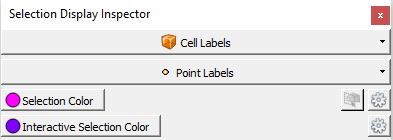
We can load the file Intro_001_Case02.xmf in ParaView to visualize any output plot file we wish. Lets select time 1.0 and lets plot Strain YY. Also we are going to activate the selection display inspector, which allow us to see the values of any variable we select for the selected elements. To do that we should go to the menu View/Selection Display Inspector. Its window will be displayed on the right of the screen as shown:

Intro_015

Selection Display Inspector window

In Cell Labels and Point Labels we can select the variables to be inspected when an element / node is selected respectively. We will click on Cell Labels and select Strain YY. Also we will click on Point Labels and select Stress YY. Then we are going to use the selection tools in ParaView to select all the elements. You can find them in small icons just above the main display window as shown here:

View and Selection Tools Icons in ParaView

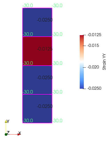
We are going to click on the icon which corresponds to "Select Cells On". Then we will click and drag with the mouse to select all the elements in the domain. Then we should be able to see some numbers on top indicating values for the inspected cell and nodal variables (black and green numbers respectively in the figure below). It should be noted that by default the colours of the inspected variables are green (cell) and yellow (point) but this can be changed by clicking on the icon next to the "Selection Color" button in the selection display inspector window. As can be seen in the figure below vertical stress (Stress YY) is -30 MPa (compressive stress because of the negative sign) in all nodes. Vertical strain in group 2 (third element from the bottom) is half of the vertical strain for the other elements because as mentioned before the Young's modulus is twice as much.

Intro_017

Inspected vertical strain and stresses at elements and nodes respectively

Concluding Remarks

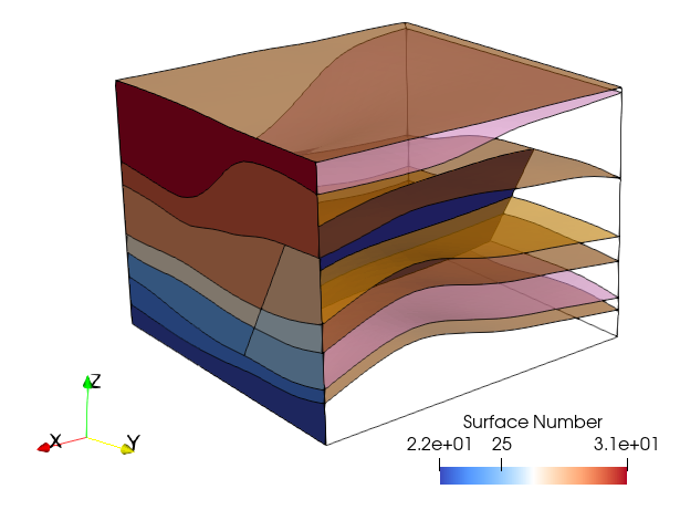
It has been shown that geometry sets are a convenient way of grouping geometry entities to be used later to assign boundary conditions. They can be also used to define groups, define stratigraphy, etc. The present example has considered a very simple geometry for demonstrative purposes but in more complex geometries which may involve multiple surfaces at boundaries, geometry sets become essential in simplifying model data definition (see for example the figure below).

Intro_014

Surfaces included in the "East" geometry set for a relatively complex geometry involving 7 stratigraphy units (top horizons shown here) and a fault.