Loading
There are several data structures relevant to defining loading and boundary conditions in ParaGeo. Those mainly are:
•Couple_freedoms to constrain the specified degrees of freedom of any field (geomechanical, flow, thermal) for all the nodes of a given geometry entity or Geometry_set so they evolve consistently (note that the constrain may be applied according to a master geometry entity or Geometry_set following a Master/Slave approach).
•Eulerian_boundary to define a geometry entity or Geometry_set as an eulerian boundary for simulating inflow/outflow of material to the system.
•Global_loads to define any time of loading (e.g. prescribed displacement, pore pressure, temperature, flow flux, etc).
•Gravity_data to apply the gravity loading.
•Load_case_control_data to define which of the Global_loads defined in the datafile are active for the simulation.
•Prescribed_boundary_data to define special prescribed displacements according to a rigid surface (Part_geometry_data).
•Stress_path_data is a boundary condition which allow to simulate burial/erosion conditions as a load applied to the domain.
•Supply_reservoir_boundary to define inflow or outflow of fluid into the system.
•Support_data to define whether a given geometry entity or Geometry_set is constrained or not.
•Transformed_freedoms to apply a rotation to the boundary conditions specified on a geometry entity or Geometry_set according to a defined local coordinate system.
•Water_level_data to apply the load corresponding to the water table to the model top surface.
•Definition of well boundary conditions via Well_definition and Well_completion data.
Note that most boundary conditions (e.g. a prescribed displacement) may have assigned a Time_curve in order to define a transient/evolutionary boundary conditions (e.g. displacement rate as a function of time).
Examples
Tutorial examples demonstrating usage of the different data structures used to apply boundary conditions to the model are:
Couple_freedoms
Eulerian_boundary
Global_loads and Load_case_control_data
Mech_001: Mechanical analysis introduction (stress load)
Cont_001: Contact example (prescribed displacement)
Val_002: Mandel's problem (prescribed pore pressure)
Gravity_data
Geost_001: Geostatic initialisation of a column
Ex_005: Sedimentation and erosion operations
Prescribed_boundary_data
Mech_003: Rift sandbox simulation using prescribed boundary data
Stress_path_data
None at present
Supply_reservoir_boundary
None at present
Support_data
Mat_003: Continuum Fracture Modelling (displacement and pore pressure)
Val_002: Mandel's problem (displacement and pore pressure)
Transformed_freedoms
None at present
Water_level
Well element boundary conditions
Ex_008 Case01: Injection and Production
Ex_008 Case02: With Contact Advection along Fault
Ex_008 Case03: U-Shaped Geothermal Well with Multiple Well Completions
Ex_008 Case04: Influence of Skin Factor on Well Elements using the Peaceman Model
Val_006: Well Geothermal - U-Shaped Closed-Loop Well System
MEM_001_Case03a: HM Coupled (High Perm Fault)
MEM_001_Case03b: HM Coupled (Low Perm Fault)
MEM_001_Case04: HM Coupled Producer and Injector Wells
MEM_001_Case04b: HM Coupled with De-activated Porous Flow Groups
MEM_001_Case04c & 04d: Implicit-Implicit HM Modelling
Overview of Well elements
Overview
The well element data structure Well_definition allows for the definition of injection, production and U-shaped wells for porous flow and thermal flow. The well path is defined through a series of points which may be "open" (leak off) or "shut"/"casing" (no leak-off). Flow within the well may be defined via injection rate, production rate or surface pore pressure with an associated time curve. For a thermal or Thermal-Hydro-Mechanical THM simulation, the temperature in the injector well may be defined as a constant well temperature or prescribed a surface temperature. For the latter case, thermal flow is solved in the well and with the surrounding rock.
The data structure can be defined when the well becomes 'live' or initially set to "shut" and later updated to "open" when the well goes 'live'. Note that for well redefinition, only the status, loading and time curve may be changed, any other changes will be ignored for the initial definition.
The Well_completion data structure details thermal properties, wall component thickness and radius for elements along a well path, linked to a specific Well_definition.
Fluid Flow
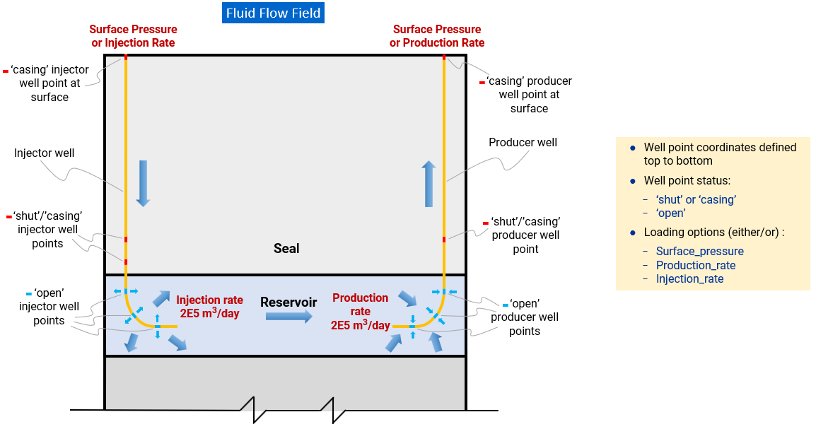
Illustration of 'Well Element' (Fluid Flow)
There are two radial flow models used to compute the pore pressure surrounding the well:
•Standard (Default) - Compute pore pressure or volumetric flow rate according to proximity interpolation factor.
•Peaceman - The Peaceman model relates well flow rate to wellblock pressure via finite-difference grid adjustments. The algorithm further updates nearby nodes with volumetric flow rate using proximity-based interpolation.
In the Standard model, the flow rate is distributed equally to the background element nodes regardless of element size.
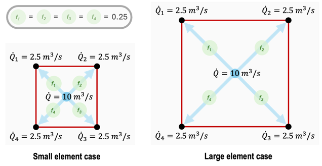
Standard Flow Model
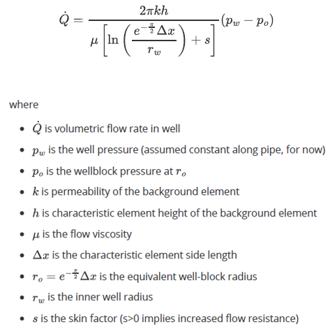
In the Peaceman model, the flow around the well is assumed to be steady-state and strictly radial in a cylindrical coordinate system. The flow rate is defined by the following equation, noting that skin factor s is also taken into consideration:
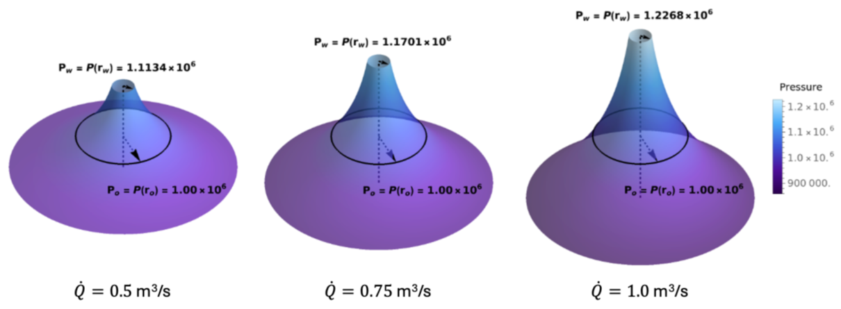
Peaceman Model: Increase of Flow Pressure Gradient with Well Injection Flow Rate
Note that the following relation leads to division by zero in the equation above

Using the calculated volumetric flow rate, each background node is updated with a value proportional to its proximity to the well node, as determined by the proximity interpolation factor ƒ.
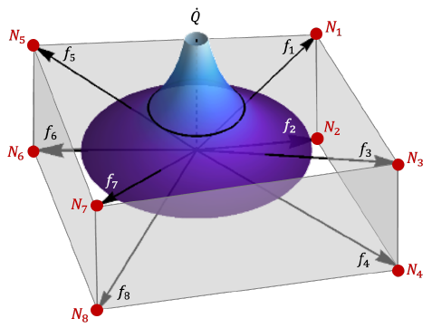
Flow is distributed to each node based on its proximity to the well, scaled by interpolation factors
Thermal Flow
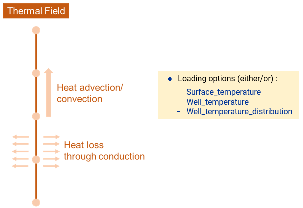
Illustration of 'Well Element' (Thermal Flow)
When temperature in the well is defined using Well_temperature or Well_temperature_distribution, these temperatures remain constant throughout the simulation, no thermal flow is solved for the well temperature.
On the other hand, if well temperature is defined using Surface_temperature, there are three radial heat models available to compute the background rock temperature distribution in a radial direction away from the well:
•Model_1 - Use far-field temperature as reference according to Ramey (1962).
•Model_2 - Use far-field temperature as reference according to Hasan (2012) (Default).
•Model_101 - Standard model using the current surrounding temperature.
In the standard Model_101, the contribution of well element to the background rock element is based on the temperature difference between the two, i.e. Twell - Trock,i.
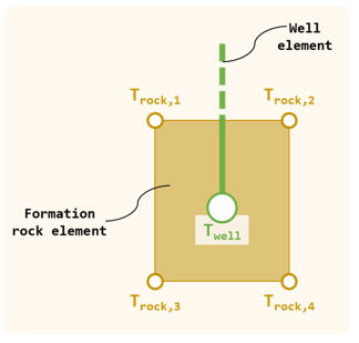
Standard "Model_101"
With the analytical approach based on the Ramey and Hasan models, the contribution of well element to the background rock element is based on the well element temperature and a fixed far-field (or initial) rock temperature. The Ramey and Hasan heat transfer equations are defined as:
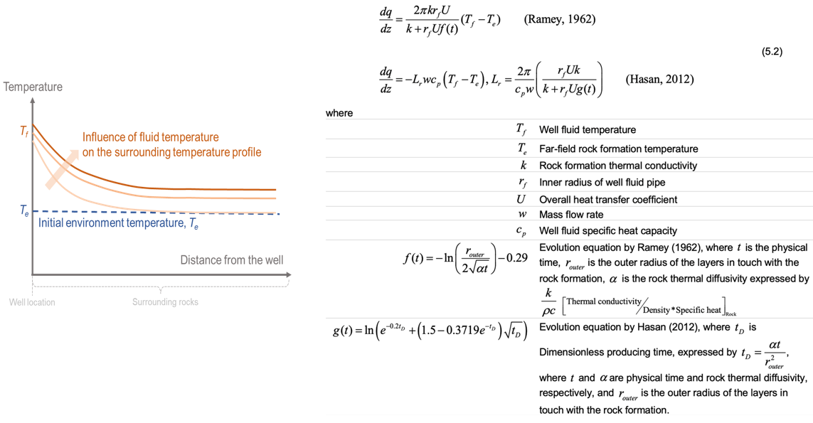
Ramey "Model_2" and Hasan "Model_1" Heat Transfer Equations
References
•Ramey, H.J., 1962, Wellbore heat transmission, Journal of Petroleum Technology
•Hasan, A.R., Kabir, S., 2012, Wellbore heat-transfer modeling and applications, Journal of Petroleum Science and Engineering
